Visualizing text data
Chapter last updated: 19 March 2025
Learning outcomes/objective: Learn…
- …about basic concepts of Natural Language Processing (NLP)
- …become familiar with a typical R-tidymodels-workflow for text analysis
- …about basic graphs for text data
Sources: Original material; Camille Landesvatter’s topic model lecture; Silge (2017)
1 Text as Data
- Many sources of text data for social scientists
- open ended survey responses, social media data, interview transcripts, news articles, official documents (public records, etc.), research publications, etc.
- even if data of interest not in textual form (yet)
- speech recognition, text recognition, machine translation etc.
- “Past”: text data often ignored (by quants), selectively read, anecdotally used or manually labeled by researchers
- Today: wide variety of text analytically methods (supervised + unsupervised) and increasing adoption of these methods by social scientists (Wilkerson and Casas 2017)
2 Language in NLP
- corpus: a collection of documents
- documents: single tweets, single statements, single text files, etc.
- tokenization: “the process of splitting text into tokens” (Silge 2017)
- tokens = single words, sequences of words or entire sentences
- Often defines the unit of analysis
- bag of words (method): approach where all tokens are put together in a “bag” without considering their order1
- possible issues with a simple bag-of-word: “I’m not happy and I don’t like it!”
- stop words: very common but uninformative terms such as “the”, “and”, “they”, etc.
- Q: Are stop words really uninformative?
- document-term/feature matrix (DTM/DFM): common format to store text data (examples later)
3 (R-)Workflow for Text Analysis
- Data collection (“Obtaining Text”*)
- Data manipulation
- Corpus pre-processing (“From Text to Data”*)
- Vectorization: Turning Text into a Matrix (DTM/DFM2) (“From Text to Data”*)
- Analysis (“Quantitative Analysis of Text”*)
- Validation and Model Selection (“Evaluating Performance”3)
- Visualization and Model Interpretation
- Visualization at descriptive and/or modelling stage
4 Data collection
- use existing corpora
- collect new corpora
- electronic sources: application user interfaces (APIs, e.g. Facebook, Twitter), web scraping, wikipedia, transcripts of all german electoral programs
- undigitized text, e.g. scans of documents
- data from interviews, surveys and/or experiments (speech → text)
- consider relevant applications to turn your data into text format (speech-to-text recognition, pdf-to-text, OCR, Mechanical Turk and Crowdflower)
5 Data manipulation
5.1 Data manipulation: Basics (1)
- Text data is different from “structured” data (e.g., a set of rows and columns)
- Most often not “clean” but rather messy
- shortcuts, dialect, incorrect grammar, missing words, spelling issues, ambiguous language, humor
- web context: emojis, # (twitter), etc.
- Preprocessing
- much more important & crucial determinant of successful text analysis!
5.2 Data manipulation: Basics (2)
Common steps in pre-processing text data:
stemming (removal of word suffixes), e.g., computation, computational, computer \(\rightarrow\) compute
lemmatisation (reduce a term to its lemma, i.e., its base form), e.g., “better” \(\rightarrow\) “good”
transformation to lower cases
removal of punctuation (e.g., ,;.-) / numbers / white spaces / URLs / stopwords / very infrequent words
\(\rightarrow\) Always choose your preprocessing steps carefully!
- e.g., removing punctuation: “I enjoy: eating, my cat and leaving out commas” vs. “I enjoy: eating my cat and leaving out commas”
Choosing unit of analysis?! (sentence vs. unigram vs. bigram etc.)
5.3 Data manipulation: Basics (3)
In principle, all those transformations can be achieved by using base R
Other packages however provide ready-to-apply functions, such as {tidytext}, {tm} or {quanteda}
Important
- transform data to corpus object or tidy text object (examples on the next slides)
6 Lab: Basic data manipulation & visualization using tidytext
6.1 Functions & packages
unnest_tokens(): split a column into tokens, flattening the table into one-token-per-row.- By default
unnest_tokens()removes punctuation and makes all terms lowercase automatically ?unnest_tokensto_lower = TRUE: Specify whether to convert tokens to lowercasedrop = TRUE: Specify whether original input column should get droppedtoken = "words": Specify unit for tokenizing, or a custom tokenizing function
- By default
anti_join(): Filtering joins filter rows from x based on the presence or absence of matches in y- e.g.,
anti_join(stopwords): Filter out stopwords
- e.g.,
cast_dtm(): Turns a “tidy” one-term-per-document-per-row data frame into a DocumentTermMatrix from thetmpackage- See also
cast_tdm()andcast_dfm() - Usage:
- See also
data_tidy %>% # Use tidy text format data
    count(text_id,word) %>% # Count words
    cast_dtm(document = text_id, # Spread into matrix
           term = word,
           value = n) %>%
as.matrix() # Store as matrix- Tidytext format lends itself to using dplyr functions
- Filter out particular tokens:
data_tidy %>%
filter(!word %in% c("t.co", "https", "rt", "http"))- Filter out 5000 rarest tokens:
tokens_rare <-
        data_tidy %>%
        count(word) %>% # Count frequency of tokens
        arrange(n) %>% # Order dataframe
        slice(1:5000) %>% # Take first 5000 rows (rarest tokens)
        pull(word) # Extract tokens

 # Filter out tokens define above
 data_tidy %>%
    filter(!word %in% tokens_rare)
6.2 Importing data & tidy text format & stop words
- Pre-processing with tidytext requires your data to be stored in a tidy text object
- Main characteristics of a tidy text dataset
- one-token-per-row
- “long format” (Row: Document \(\times\) token)
First, we have to retrieve some data. We’ll use tweet data from Russian trolls (Roeder 2018) (these are not real people anyways). The data below is edited data (variables & observations subsampled, language == English, account_category == LeftTroll or RightTroll) based on the file IRAhandle_tweets_1.csv. The variables are explained here: https://github.com/fivethirtyeight/russian-troll-tweets/.
Below we start by installing/loading the necessary packages:
Then we load the data into R (use the link on your computer):
[1] 4000 9We start by adding an identifier text_id to the documents/tweets.
| text_id | author | text | region | language | publish_date | following | followers | account_type | account_category |
|---|---|---|---|---|---|---|---|---|---|
| 1 | AMELIEBALDWIN | ‘(GenFlynn?) (realDonaldTrump?) (mike_pence?) after what I witnessed today… wis needs serious help! Anti worker anti liberty agenda. Elite B.S. https://t.co/URL3FrNfqT’ | United States | English | 10/9/2016 4:45 | 1944 | 2472 | Right | RightTroll |
| 2 | ACEJINEV | Trans-Siberian Orchestra Tickets On Sale. Buy #TSO Christmas Concert #Tickets (eCityTickets?) https://t.co/FWMaOWxEh7 https://t.co/J2ZzUe87Fl | United States | English | 11/7/2016 14:54 | 803 | 908 | Left | LeftTroll |
| 3 | ANDEERLWR | #anderr GRAPHIC VIDEO : Did ANTIFA Violence Cause the Tragedy at #Charlottesville? https://t.co/y2QeK4AC0J https://t.co/OEXcWQdiL4 | United States | English | 8/13/2017 16:47 | 21 | 6 | Right | RightTroll |
| 4 | AMELIEBALDWIN | Remember all the fuss when the US wrongly accused #Russia of destroying hospitals in #Syria? Well this is for real https://t.co/U5LHrZLgnB | United States | English | 3/18/2017 20:22 | 2303 | 2744 | Right | RightTroll |
| 5 | ALBERTMORENMORE | RT (2AFight?): More people die from alcohol than guns. READ> https://t.co/7H6OlJJtEC #2A #NRA #tcot #tgdn #PJNET #ccot #teaparty https://t.c… | United States | English | 2/18/2016 9:02 | 1136 | 729 | Right | RightTroll |
| 6 | AMELIEBALDWIN | ‘(RealAlexJones?) (BarackObama?) (POTUS?) (theDemocrats?) Obama is the Divider-In-Chief. His mission from Soros was destroy America from within.’ | United States | English | 11/30/2016 8:25 | 2366 | 2578 | Right | RightTroll |
[1] 4000 10Then, by using the unnest_tokens() function from tidytext we transform this data to a tidy text format, where the words (tokens) of each text/document are written into their own rows.
| text_id | author | text | word | region | language | publish_date | following | followers | account_type | account_category |
|---|---|---|---|---|---|---|---|---|---|---|
| 1 | AMELIEBALDWIN | ‘(GenFlynn?) (realDonaldTrump?) (mike_pence?) after what I witnessed today… wis needs serious help! Anti worker anti liberty agenda. Elite B.S. https://t.co/URL3FrNfqT’ | genflynn | United States | English | 10/9/2016 4:45 | 1944 | 2472 | Right | RightTroll |
| 1 | AMELIEBALDWIN | ‘(GenFlynn?) (realDonaldTrump?) (mike_pence?) after what I witnessed today… wis needs serious help! Anti worker anti liberty agenda. Elite B.S. https://t.co/URL3FrNfqT’ | realdonaldtrump | United States | English | 10/9/2016 4:45 | 1944 | 2472 | Right | RightTroll |
| 1 | AMELIEBALDWIN | ‘(GenFlynn?) (realDonaldTrump?) (mike_pence?) after what I witnessed today… wis needs serious help! Anti worker anti liberty agenda. Elite B.S. https://t.co/URL3FrNfqT’ | mike_pence | United States | English | 10/9/2016 4:45 | 1944 | 2472 | Right | RightTroll |
| 1 | AMELIEBALDWIN | ‘(GenFlynn?) (realDonaldTrump?) (mike_pence?) after what I witnessed today… wis needs serious help! Anti worker anti liberty agenda. Elite B.S. https://t.co/URL3FrNfqT’ | witnessed | United States | English | 10/9/2016 4:45 | 1944 | 2472 | Right | RightTroll |
| 1 | AMELIEBALDWIN | ‘(GenFlynn?) (realDonaldTrump?) (mike_pence?) after what I witnessed today… wis needs serious help! Anti worker anti liberty agenda. Elite B.S. https://t.co/URL3FrNfqT’ | wis | United States | English | 10/9/2016 4:45 | 1944 | 2472 | Right | RightTroll |
| 1 | AMELIEBALDWIN | ‘(GenFlynn?) (realDonaldTrump?) (mike_pence?) after what I witnessed today… wis needs serious help! Anti worker anti liberty agenda. Elite B.S. https://t.co/URL3FrNfqT’ | anti | United States | English | 10/9/2016 4:45 | 1944 | 2472 | Right | RightTroll |
[1] 44001 11- Questions:
- How does our dataset change after tokenization and removing stopwords? How many observations do we now have? And what do the variable
text_idandwordidentify/store? - Also, have a closer look at the single words. Do you notice anything else that has changed, e.g., is something missing from the original text?
- How does our dataset change after tokenization and removing stopwords? How many observations do we now have? And what do the variable
We can use str() and data_tidy$word[1:15] to inspect the resulting data/tokens.
tibble [44,001 × 11] (S3: tbl_df/tbl/data.frame)
$ text_id : int [1:44001] 1 1 1 1 1 1 1 1 1 1 ...
$ author : chr [1:44001] "AMELIEBALDWIN" "AMELIEBALDWIN" "AMELIEBALDWIN" "AMELIEBALDWIN" ...
$ text : chr [1:44001] "'@GenFlynn @realDonaldTrump @mike_pence after what I witnessed today... wis needs serious help! Anti worker ant"| __truncated__ "'@GenFlynn @realDonaldTrump @mike_pence after what I witnessed today... wis needs serious help! Anti worker ant"| __truncated__ "'@GenFlynn @realDonaldTrump @mike_pence after what I witnessed today... wis needs serious help! Anti worker ant"| __truncated__ "'@GenFlynn @realDonaldTrump @mike_pence after what I witnessed today... wis needs serious help! Anti worker ant"| __truncated__ ...
$ word : chr [1:44001] "genflynn" "realdonaldtrump" "mike_pence" "witnessed" ...
$ region : chr [1:44001] "United States" "United States" "United States" "United States" ...
$ language : chr [1:44001] "English" "English" "English" "English" ...
$ publish_date : chr [1:44001] "10/9/2016 4:45" "10/9/2016 4:45" "10/9/2016 4:45" "10/9/2016 4:45" ...
$ following : num [1:44001] 1944 1944 1944 1944 1944 ...
$ followers : num [1:44001] 2472 2472 2472 2472 2472 ...
$ account_type : chr [1:44001] "Right" "Right" "Right" "Right" ...
$ account_category: chr [1:44001] "RightTroll" "RightTroll" "RightTroll" "RightTroll" ... [1] "genflynn" "realdonaldtrump" "mike_pence" "witnessed"
[5] "wis" "anti" "worker" "anti"
[9] "liberty" "agenda" "elite" "b.s"
[13] "https" "t.co" "url3frnfqt" 6.3 Data manipulation: Tidytext Example (2)
- Other transformations may need some dealing with regular expressions
- e.g., to remove white space with tidytext (
s+describes a blank space):
- e.g., to remove white space with tidytext (
[1] "'@GenFlynn@realDonaldTrump@mike_penceafterwhatIwitnessedtoday...wisneedsserioushelp!Antiworkerantilibertyagenda.EliteB.S.https://t.co/URL3FrNfqT'"
[2] "Trans-SiberianOrchestraTicketsOnSale.Buy#TSOChristmasConcert#Tickets@eCityTicketshttps://t.co/FWMaOWxEh7https://t.co/J2ZzUe87Fl"
[3] "#anderrGRAPHICVIDEO:DidANTIFAViolenceCausetheTragedyat#Charlottesville?https://t.co/y2QeK4AC0Jhttps://t.co/OEXcWQdiL4"
[4] "RememberallthefusswhentheUSwronglyaccused#Russiaofdestroyinghospitalsin#Syria?Wellthisisforrealhttps://t.co/U5LHrZLgnB"
[5] "RT@2AFight:Morepeoplediefromalcoholthanguns.READ>https://t.co/7H6OlJJtEC#2A#NRA#tcot#tgdn#PJNET#ccot#teapartyhttps://t.c…" - Advantage: tidy text format → regular R functions can be used
- …instead of functions specialized to analyze a corpus object
- e.g., use dplyr workflow to count the most popular words in your text data:
Below an example where we first identify the rarest tokens and then filter them out:
# Identify rare tokens
tokens_rare <-
data_tidy %>%
count(word) %>% # Count frequency of tokens
arrange(n) %>% # Order dataframe
slice(1:5000) %>% # Take first 5000 rows (rarest tokens)
pull(word) # Extract tokens
# Filter out tokens define above
data_tidy_filtered <-
data_tidy %>%
filter(!word %in% tokens_rare)
dim(data_tidy_filtered)[1] 39001 11- Tidytext is a good starting point (in my opinion), because we (can) carry out these steps individually
- other packages combine many steps into one single function (e.g. quanteda combines pre-processing and DFM casting in one step)
- R (as usual) offers many ways to achieve similar or same results
- e.g. you could also import, filter and pre-process using dplyr and tidytext, further pre-process and vectorize with tm or quanteda (tm has simpler grammar but slightly fewer features), use machine learning applications and eventually re-convert to tidy format for interpretation and visualization (ggplot2)
7 Vectorization: Basics
- Text analytical models (e.g., topic models) often require the input data to be stored in a certain format
- Typically: document-term matrix (DTM), sometimes also called document-feature matrix (DFM)
- turn raw text into a vector-space representation
- matrix where each row represents a document and each column represents a word
- term-frequency (tf): the number within each cell describes the number of times the word appears in the document
- term frequency–inverse document frequency (tf-idf): weights occurrence of certain words, e.g., lowering weight of word “education” in corpus of articles on educational inequality
8 Lab: Vectorization with Tidytext
Repeat all the steps from above…
# load and install packages if neccessary
# install.packages(pacman)
pacman::p_load(tidyverse,
                             rvest,
                             xml2,
                             tidytext,
                             tm,
                             ggwordcloud,
                             knitr)
# Load the data
# data_IRAhandle_tweets_1_sampled.csv
# data <- read_csv(sprintf("https://docs.google.com/uc?id=%s&export=download",
#                          "1GNrZfF3itKxUtbngQhP6lCyOM3ApbgTD"))


data <- read_csv("data/data_IRAhandle_tweets_1_sampled.csv",
                 col_types = cols())
dim(data) # What dimensions do we have?
[1] 4000 9# Add id
data <- data %>%
mutate(text_id = row_number()) %>%
select(text_id, everything()) # What happens here?
# Create tidy text format and remove stopwords
data_tidy <- data %>%
unnest_tokens(word, text, drop = FALSE) %>%
anti_join(stop_words) %>%
select(text_id, author, text, word, everything())
kable(head(data_tidy))| text_id | author | text | word | region | language | publish_date | following | followers | account_type | account_category |
|---|---|---|---|---|---|---|---|---|---|---|
| 1 | AMELIEBALDWIN | ‘(GenFlynn?) (realDonaldTrump?) (mike_pence?) after what I witnessed today… wis needs serious help! Anti worker anti liberty agenda. Elite B.S. https://t.co/URL3FrNfqT’ | genflynn | United States | English | 10/9/2016 4:45 | 1944 | 2472 | Right | RightTroll |
| 1 | AMELIEBALDWIN | ‘(GenFlynn?) (realDonaldTrump?) (mike_pence?) after what I witnessed today… wis needs serious help! Anti worker anti liberty agenda. Elite B.S. https://t.co/URL3FrNfqT’ | realdonaldtrump | United States | English | 10/9/2016 4:45 | 1944 | 2472 | Right | RightTroll |
| 1 | AMELIEBALDWIN | ‘(GenFlynn?) (realDonaldTrump?) (mike_pence?) after what I witnessed today… wis needs serious help! Anti worker anti liberty agenda. Elite B.S. https://t.co/URL3FrNfqT’ | mike_pence | United States | English | 10/9/2016 4:45 | 1944 | 2472 | Right | RightTroll |
| 1 | AMELIEBALDWIN | ‘(GenFlynn?) (realDonaldTrump?) (mike_pence?) after what I witnessed today… wis needs serious help! Anti worker anti liberty agenda. Elite B.S. https://t.co/URL3FrNfqT’ | witnessed | United States | English | 10/9/2016 4:45 | 1944 | 2472 | Right | RightTroll |
| 1 | AMELIEBALDWIN | ‘(GenFlynn?) (realDonaldTrump?) (mike_pence?) after what I witnessed today… wis needs serious help! Anti worker anti liberty agenda. Elite B.S. https://t.co/URL3FrNfqT’ | wis | United States | English | 10/9/2016 4:45 | 1944 | 2472 | Right | RightTroll |
| 1 | AMELIEBALDWIN | ‘(GenFlynn?) (realDonaldTrump?) (mike_pence?) after what I witnessed today… wis needs serious help! Anti worker anti liberty agenda. Elite B.S. https://t.co/URL3FrNfqT’ | anti | United States | English | 10/9/2016 4:45 | 1944 | 2472 | Right | RightTroll |
With the cast_dtm function from the tidytext package, we can now transform it to a DTM.
[1] 4000 15151 Terms
Docs agenda anti b.s elite genflynn https
1 1 2 1 1 1 1
2 0 0 0 0 0 2
3 0 0 0 0 0 2
4 0 0 0 0 0 1
5 0 0 0 0 0 2
6 0 0 0 0 0 09 Lab: Text visualization
Repeat all the steps from above…
# load and install packages if neccessary
# install.packages(pacman)
pacman::p_load(tidyverse,
                             rvest,
                             xml2,
                             tidytext,
                             tm,
                             ggwordcloud)

# Load the data
# data_IRAhandle_tweets_1_sampled.csv
# data <- read_csv(sprintf("https://docs.google.com/uc?id=%s&export=download",
#                          "1GNrZfF3itKxUtbngQhP6lCyOM3ApbgTD"))


data <- read_csv("data/data_IRAhandle_tweets_1_sampled.csv",
                 col_types = cols())


# Add id
data <- data %>%
                mutate(text_id = row_number()) %>%
                select(text_id, everything()) # What happens here?


# Create tidy text format and remove stopwords
data_tidy <- data %>%
  unnest_tokens(word, text, drop = FALSE) %>%
  anti_join(stop_words) %>%
    select(text_id, author, text, word, everything())
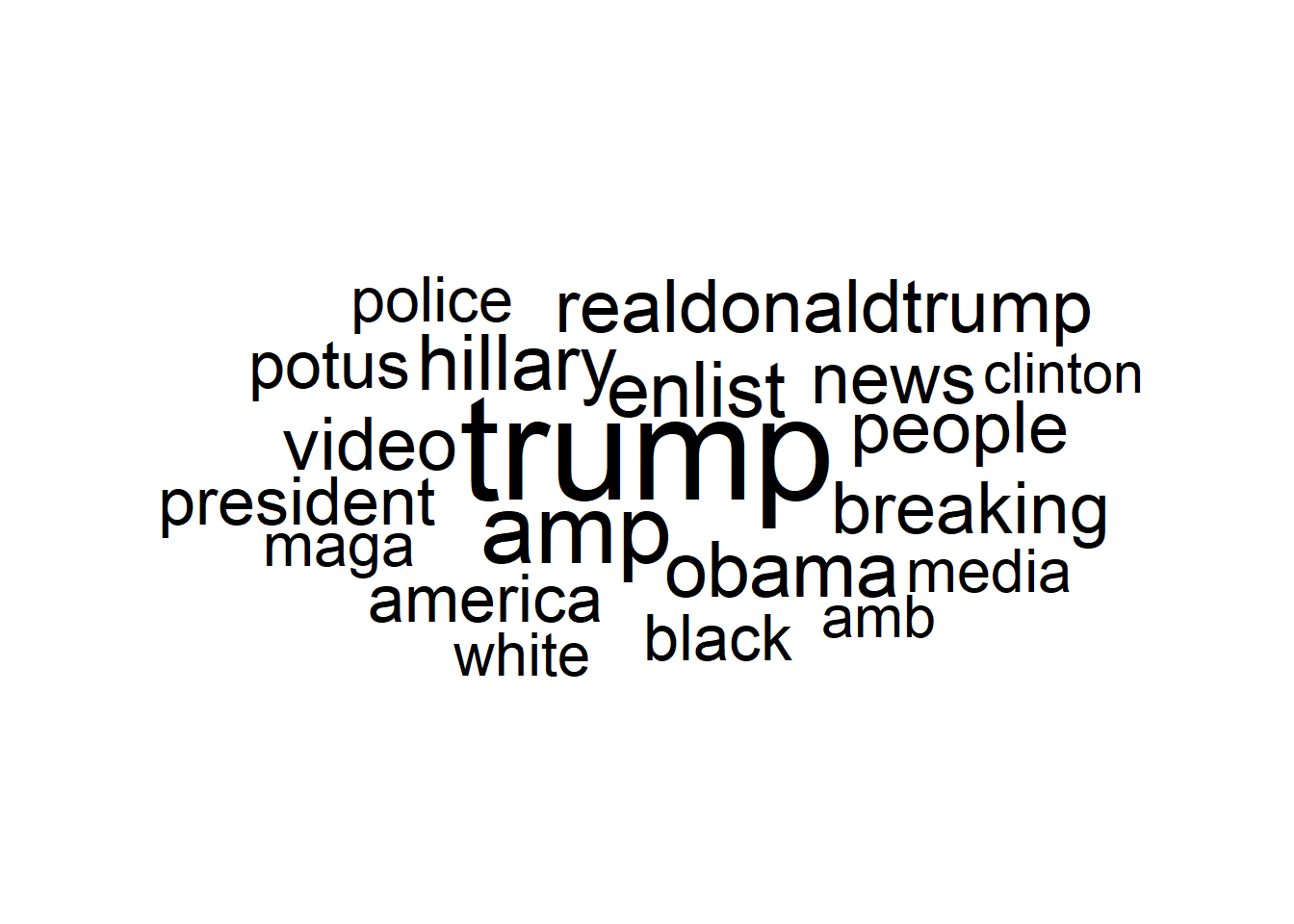
9.1 Wordclouds
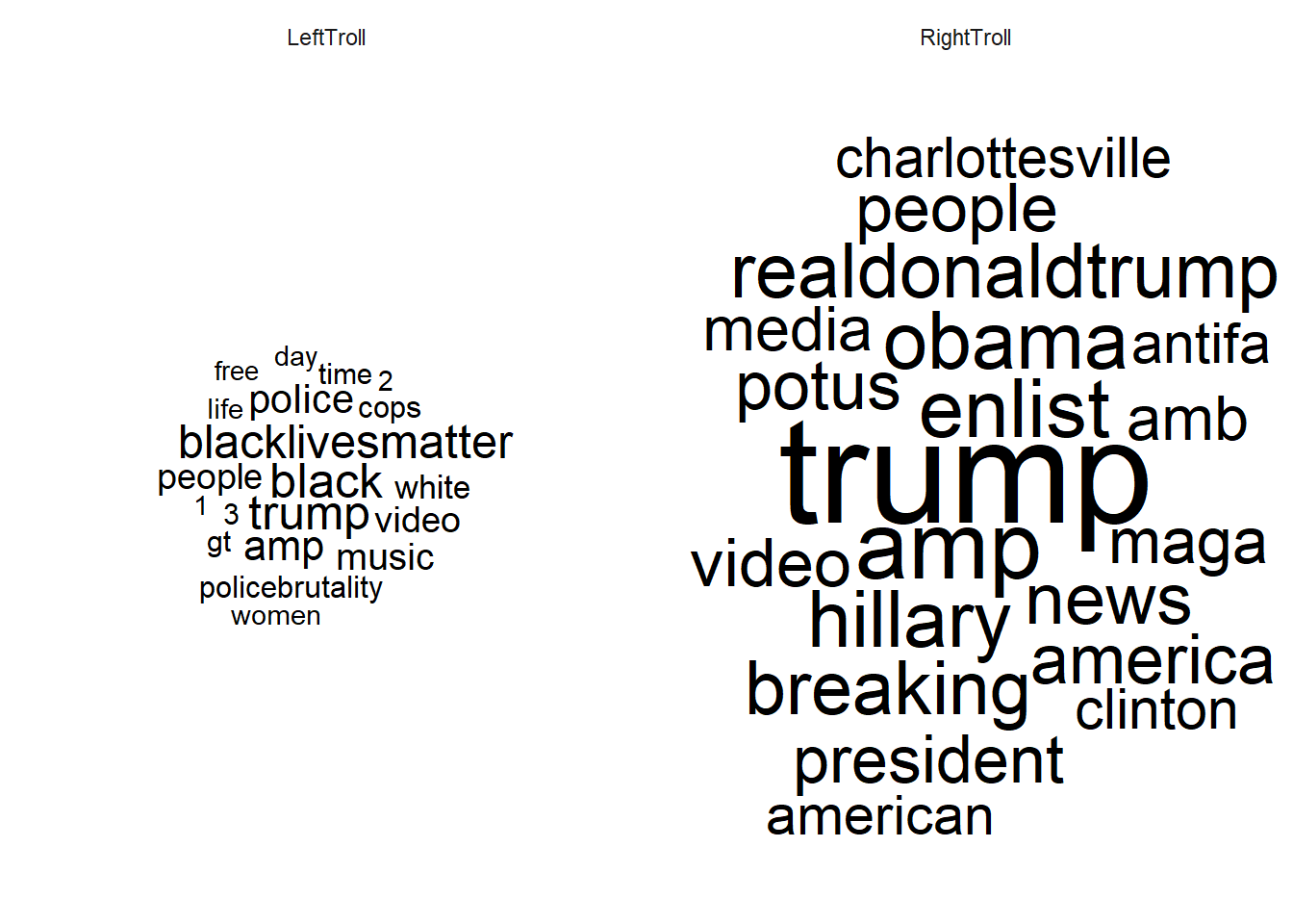
9.2 Wordclouds across subsets (grouped)
set.seed(42)


# Aggregate by word
data_plot <- data_tidy %>%
    filter(!word %in% c("t.co", "https", "rt", "http")) %>%
    count(word, account_category) %>%
    group_by(account_category) %>%
    arrange(desc(n)) %>%
    slice(1:20) %>%
    ungroup()

# Wordcloud: Coloring different groups
ggplot(data_plot, aes(label = word, size = n, color = account_category)) +
  geom_text_wordcloud() +
  scale_size_area(max_size = 20) +
  theme_minimal()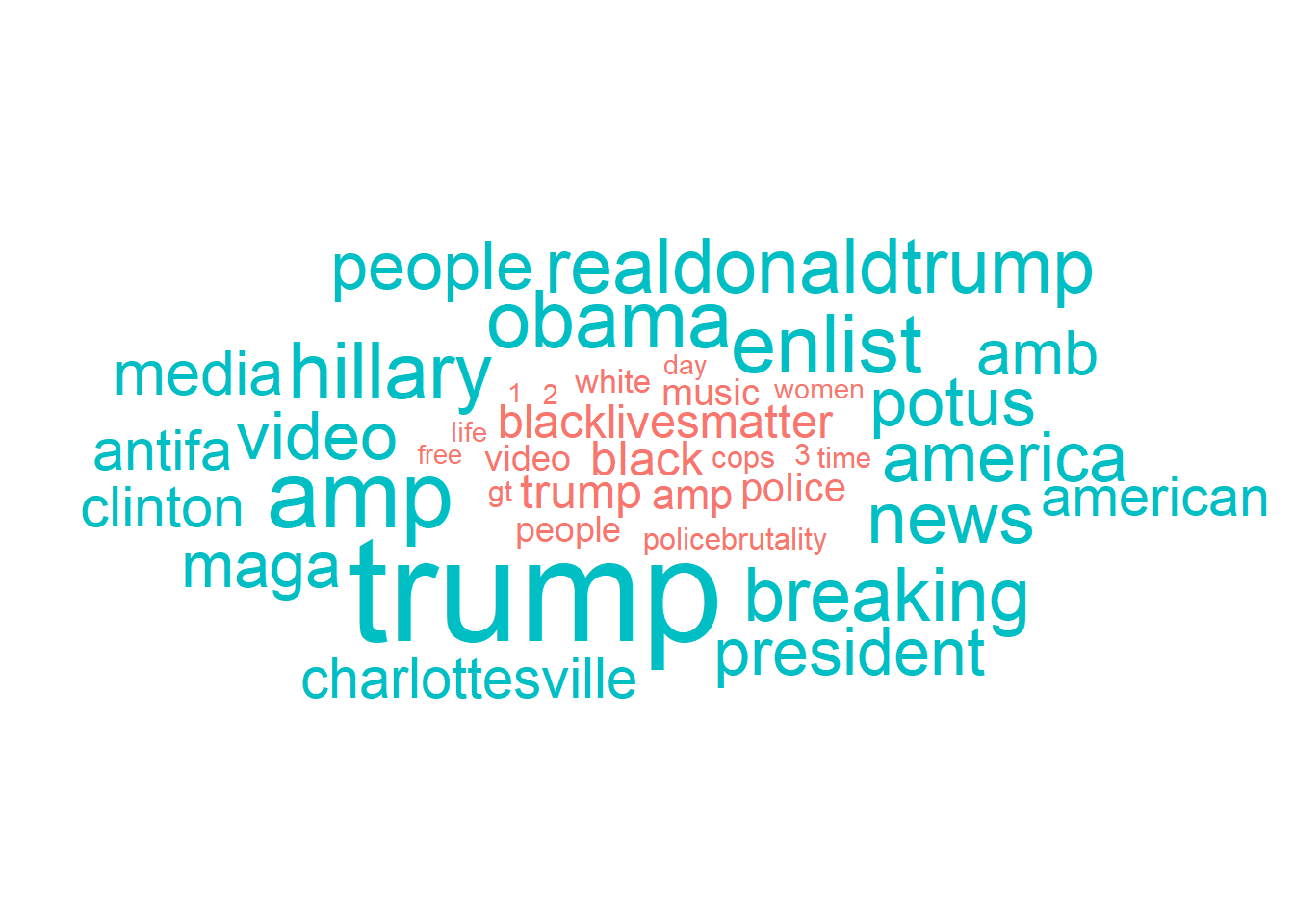
9.3 Barplots (Frequency)
set.seed(42)


# Data for vertical barplot
data_plot <-
    data_tidy %>%
    filter(!word %in% c("t.co", "https", "rt", "http")) %>%
    group_by(word) %>%
  summarize(n= n()) %>%
    arrange(desc(n)) %>%
    slice(1:10) %>%
    mutate(word = factor(word, # Convert to factor for ordering
                                             levels = as.character(.$word),
                                             ordered = TRUE))


# Create barplot
ggplot(data_plot, aes(x = word, y = n)) +
  geom_bar(stat="identity") +
  theme_minimal() +
    theme(axis.text.x = element_text(angle = 45, hjust = 1))
# Data for horizontal barplot
data_plot <- data_plot %>%
    arrange(n) %>%
    mutate(word = factor(word,
                                             levels = as.character(.$word),
                                             ordered = TRUE))

# Create horizontal barplot
ggplot(data_plot, aes(x = n, y = word)) +
  geom_bar(stat="identity") +
  theme_minimal() +
    theme(axis.text.y = element_text(angle = 45, hjust = 1))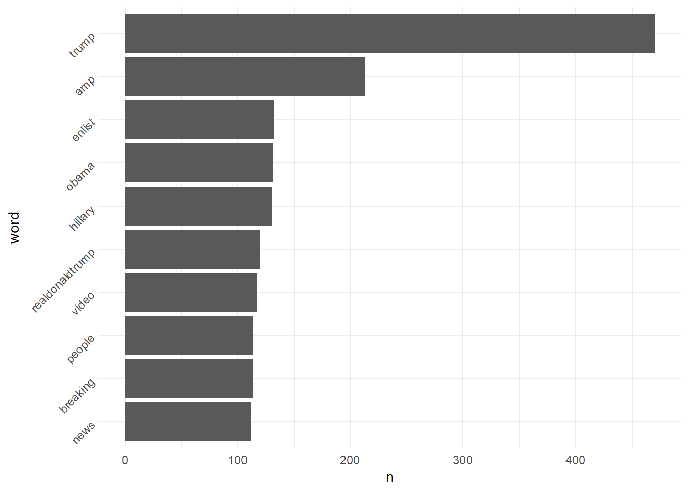
# Data for faceted horizontal barplot
data_plot <-
    data_tidy %>%
    filter(!word %in% c("t.co", "https", "rt", "http")) %>%
    group_by(word, account_category) %>%
  summarize(n= n(),
                    account_category = first(account_category)) %>%
    group_by(account_category) %>%
    arrange(desc(n)) %>%
    slice(1:10) %>%
    ungroup()


# Create horizontal barplot
ggplot(data_plot, aes(x = n, y = word)) +
  geom_bar(stat="identity") +
  theme_minimal() +
    theme(axis.text.y = element_text(angle = 45, hjust = 1)) +
  facet_wrap(~account_category)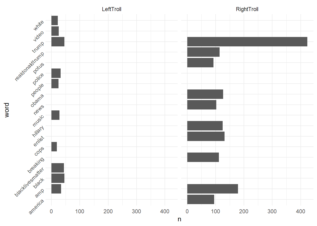
10 TM example: Text pre-processing and vectorization
- \(\rightarrow\) consider alternative packages (e.g., tm, quanteda)
- Example: tm package
- input: corpus not tidytext object
- What is a corpus in R? \(\rightarrow\) group of documents with associated metadata
# Load the data
# data_IRAhandle_tweets_1_sampled.csv
# data <- read_csv(sprintf("https://docs.google.com/uc?id=%s&export=download",
#                          "1GNrZfF3itKxUtbngQhP6lCyOM3ApbgTD"))


data <- read_csv("data/data_IRAhandle_tweets_1_sampled.csv",
                 col_types = cols())

data <- data %>%
                mutate(text_id = row_number()) %>%
                select(text_id, everything())
dim(data)
# Clean corpus
corpus_clean <- VCorpus(VectorSource(data$text)) %>%
tm_map(removePunctuation, preserve_intra_word_dashes = TRUE) %>%
tm_map(removeNumbers) %>%
tm_map(content_transformer(tolower)) %>%
tm_map(removeWords, words = c(stopwords("en"))) %>%
tm_map(stripWhitespace) %>%
tm_map(stemDocument)
# Check exemplary document
corpus_clean[["1"]][["content"]][1] "genflynn realdonaldtrump mikep wit today wis need serious help anti worker anti liberti agenda elit bs httpstcourlfrnfqt"- In case you pre-processed your data with the tm package, remember we ended with a pre-processed corpus object
- Now, simply apply the DocumentTermMatrix function to this corpus object
<<DocumentTermMatrix (documents: 4000, terms: 6)>>
Non-/sparse entries: 9/23991
Sparsity           : 100%
Maximal term length: 12
Weighting          : term frequency (tf)
Sample             :
      Terms
Docs   ����� ������ ꮮꭺꮖꭼ ꮑꭵꮆꮋꮖ ꭶꮎ� ������������
  1        0      0    0     0   0            0
  1640     1      0    0     0   0            0
  2        0      0    0     0   0            0
  2869     0      0    0     0   0            1
  2889     0      1    0     0   0            0
  3        0      0    0     0   0            0
  3509     0      0    1     1   1            0
  3534     1      0    0     0   0            0
  640      1      0    0     0   0            0
  884      0      1    0     0   0            0
Q: How do the terms between the DTM we created with tidytext and the one created with tm differ? Why?
References
Footnotes
Alternatives: bigrams/word pairs, word embeddings↩︎
Document-term matrix (DTM) is a mathematical representation of text data where rows correspond to documents in the corpus, and columns correspond to terms (words or phrases). DFM, also known as a document-feature matrix, is similar to a DTM but instead of representing the count of terms in each document, it represents the presence or absence of terms.↩︎
