library(tidyverse)library(modelsummary)# data_twitter_influence.csv# data <- read_csv(sprintf("https://docs.google.com/uc?id=%s&export=download",# "1dLSTUJ5KA-BmAdS-CHmmxzqDFm2xVfv6"))data <- readr::read_csv("data/data_twitter_influence.csv",col_types =cols())# Numeric datadatasummary_skim(data, type ="numeric", output ="html")
Unique
Missing Pct.
Mean
SD
Min
Median
Max
Histogram
n_retweets
237
0
429.4
2332.7
0.0
36.0
48568.0
followers_count
485
0
13184.0
51672.6
12.0
2647.5
693125.0
account_age_months
504
0
84.1
40.7
5.0
87.3
143.6
account_age_years
504
0
7.0
3.4
0.4
7.3
12.0
female
2
0
0.3
0.5
0.0
0.0
1.0
# Categorical data (we had to create)datasummary_skim(data %>%mutate(party =factor(party),female =factor(female)), type ="categorical", output ="html")
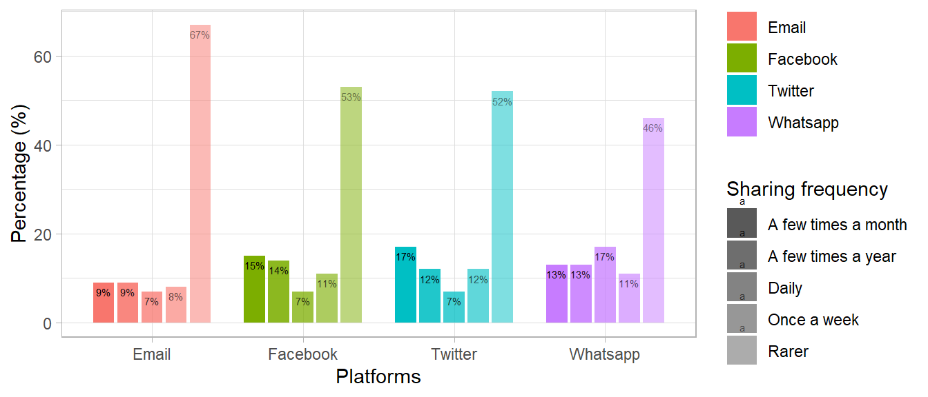
Figure 1: Distribution of four categorical variables
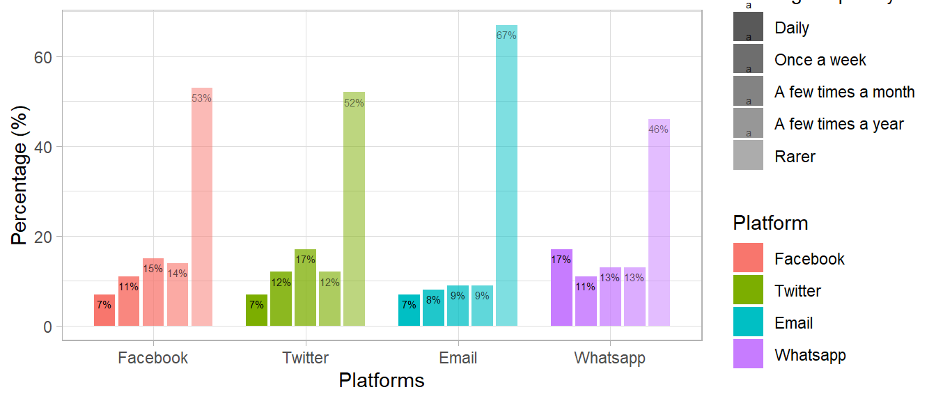
Rename the category names:
data_plot <- data_plot %>%mutate(variable =recode(variable,"sharing_email"="Email","sharing_fb"="Facebook","sharing_twitter"="Twitter","sharing_whatsapp"="Whatsapp"),category =recode(category,"pct.Seltener"="Rarer","pct.EinpaarMalimJahr"="A few times a year", "pct.EinpaarMalimMonat"="A few times a month", "pct.EinmalproWoche"="Once a week","pct.Taeglich"="Daily"))str(data_plot)
data_plot$category <-factor(data_plot$category, levels =c("Daily", "Once a week", "A few times a month", "A few times a year", "Rarer"))levels(data_plot$category)
[1] "Daily"               "Once a week"         "A few times a month"
[4] "A few times a year"  "Rarer"
tidyr::expand(): To create observations/rows for non-observed variable combinations
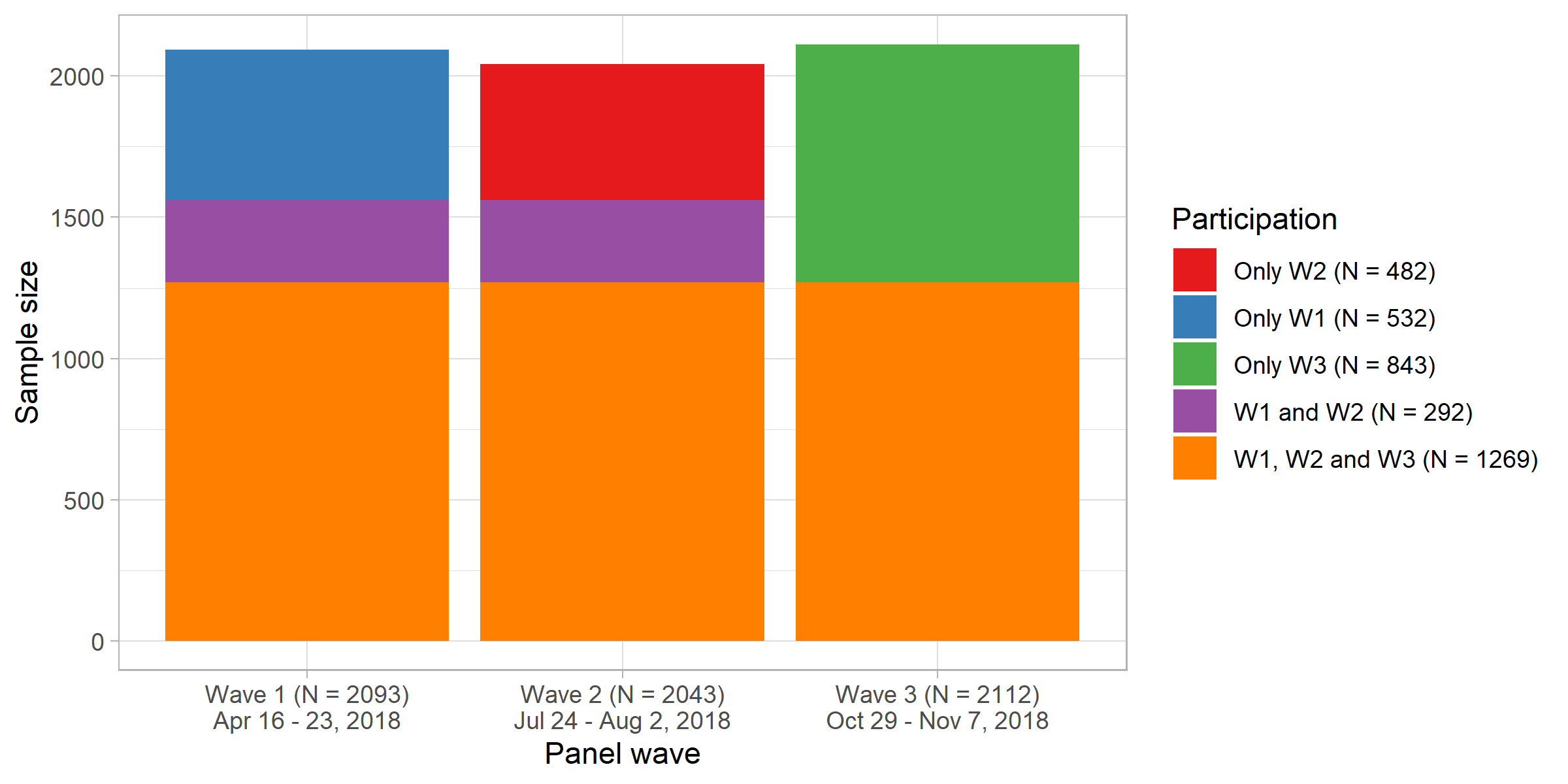
2.3.2 Graph
Here we’ll reproduce and maybe criticize as well as improve Figure @ref(fig:fig-participation-across-waves) (Bauer et al. 2020)
Questions:
What does the graph show? What are the underlying variables (and data)?
How many scales/mappings does it use? Could we reduce them?
What do you like, what do you dislike about the figure? What is good, what is bad?
What kind of information could we add to the graph (if any)?
How would you approach a replication of the graph?
Figure 4: Presence/participation at/in different time points/waves
2.3.3 Lab: Data & Code
The code for Figure @ref(fig:fig-participation-across-waves) is shown below (and creates Figure @ref(fig:fig-participation-across-waves2)).
Learning objectives
How to make stacked barplots
How to expand data
We’ll start by preparing the data for our plot. As you can see below the data is in long-format already and contains an individual identifier pid as well as two variables that contain the same information namely the wave identifier in different format: wave.num and wave.
If you want directly move to the plot…
# data_wave_participation.csv# data <- read_csv(sprintf("https://docs.google.com/uc?id=%s&export=download",# "1Y9z1shAjyaHgqpOxwt2T8uSoe-3RW-WI"),# col_types = cols())data <-read_csv("data/data_wave_participation.csv")head(data)
We expand the data creating a new dataframe that we join with the older one. Like that we end up with a dataframe that indicated missings for missing \(\times\) respondent wave observations.
# Expand to get dataset with rows for non observationsdata.expand <- data %>% tidyr::expand(pid, wave.num)head(data.expand)
# Right_Join with longformat data to real presence of respondentsdata.expand <- data %>%right_join(data.expand) %>%arrange(pid, wave.num)head(data.expand)
Subsequently, we have to pursue different steps to summarize the data across waves as well as delete the categories with the smallest numbers (participants only in W2/W3 (N = 3) and only in W1/W3 (N = 2)). If you like you can skip this whole part and directly go to the function below.
# Subset variables#data.expand <- data.expand %>% select(pid, wave.num, wave) # %>% distinct()# Spread dataset and arrangedata.expand <- data.expand %>%pivot_wider(names_from = wave.num, values_from = wave) %>%arrange(pid)# Rename wave variablesdata.expand <-rename(data.expand, wave1 ="1", wave2 ="2", wave3 ="3")# Create "across_waves" with information of presence in single wavesdata.expand <-unite(data.expand, across_waves, -pid)# Aggregate to get observations per presence in different wavesdata.expand <- data.expand %>%group_by(across_waves) %>%summarize(n =n())# Separate united variabledata.expand <- data.expand %>%separate(across_waves, c("Wave1", "Wave2", "Wave3"), sep ="_")# Replace values of wave variables with N valuesdata.expand$Wave1[data.expand$Wave1 !="NA"] <- data.expand$n[data.expand$Wave1 !="NA"]data.expand$Wave2[data.expand$Wave2 !="NA"] <- data.expand$n[data.expand$Wave2 !="NA"]data.expand$Wave3[data.expand$Wave3 !="NA"] <- data.expand$n[data.expand$Wave3 !="NA"]# Delete groups only W2/W3 (N = 3) and only W1/W3 (N = 2)data.expand <- data.expand %>%filter(n >5) %>%select(-n)# Create barplot illustrating the sampels across wavesdata.expand <-pivot_longer(data.expand, Wave1:Wave3, names_to ="wave", values_to ="samples")data.expand$samples <-as.numeric(data.expand$samples)data.expand$samples_labels <- dplyr::recode(data.expand$samples,"532"="Only W1 (N = 532)","292"="W1 and W2 (N = 292)","1269"="W1, W2 and W3 (N = 1269)","482"="Only W2 (N = 482)","843"="Only W3 (N = 843)")data.expand <- data.expand %>%filter(!is.na(samples))data.expand <- data.expand %>%arrange(wave)data_plot <- data.expanddata_plot
# A tibble: 8 × 3
  wave  samples samples_labels
  <chr>   <dbl> <chr>
1 Wave1     532 Only W1 (N = 532)
2 Wave1     292 W1 and W2 (N = 292)
3 Wave1    1269 W1, W2 and W3 (N = 1269)
4 Wave2     482 Only W2 (N = 482)
5 Wave2     292 W1 and W2 (N = 292)
6 Wave2    1269 W1, W2 and W3 (N = 1269)
7 Wave3     843 Only W3 (N = 843)
8 Wave3    1269 W1, W2 and W3 (N = 1269)
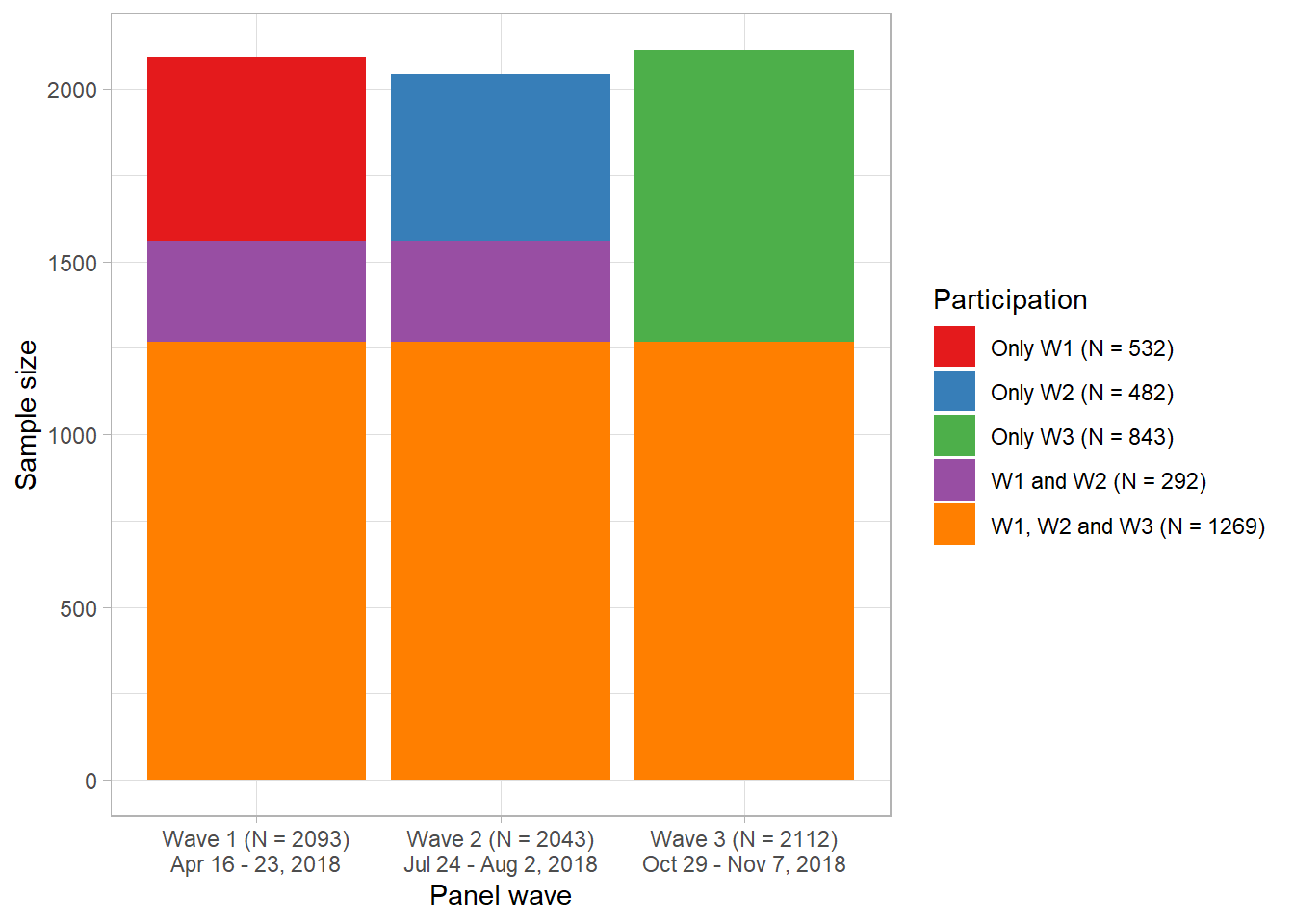
Finally, we plot the participation across waves in Figure @ref(fig:fig-participation-across-waves2).
Figure 5: Presence/participation at/in different time points/waves
2.3.4 Exercise
Try to produce such a graph with a panel survey that you are currently using. Store the panel data in long-format, only keep the participant ID as well as the wave number, rename these pid and wave.num and then start with the code.
2.4 Another animation
Bauer, Paul C, Frederic Gerdon, Florian Keusch, and Frauke Kreuter. 2020. “The Impact of the GDPR Policy on Data Sharing/Privacy Attitudes.”Preliminary Draft, 1–22.