| id | name | compas_screening_date | reoffend | reoffend_factor | age | priors_count |
|---|---|---|---|---|---|---|
| 1 | miguel hernandez | 2013-08-14 | 0 | no | 69 | 0 |
| 3 | kevon dixon | 2013-01-27 | 1 | yes | 34 | 0 |
| 4 | ed philo | 2013-04-14 | 1 | yes | 24 | 4 |
| 5 | marcu brown | 2013-01-13 | 0 | no | 23 | 1 |
| 6 | bouthy pierrelouis | 2013-03-26 | 0 | no | 43 | 2 |
| 7 | marsha miles | 2013-11-30 | 0 | no | 44 | 0 |
| 8 | edward riddle | 2014-02-19 | 1 | yes | 41 | 14 |
| 9 | steven stewart | 2013-08-30 | NA | NA | 43 | 3 |
| 10 | elizabeth thieme | 2014-03-16 | 0 | no | 39 | 0 |
| 13 | bo bradac | 2013-11-04 | 1 | yes | 21 | 1 |
Classification: Logistic model
Chapter last updated: 12 Februar 2025
Learning outcomes/objective: Learn…
- …and repeat logic underlying logistic model.
- …how to assess accuracy in classification (logistic regression).
- …concepts (training dataset etc.) using a “simple example”.
1 Predicting Recidvism: The data
Table 1 depicts the first rows/columns of the dataset (COMPAS) we use.
2 Predicting Recidvism: Background story
- Background story by ProPublica: Machine Bias
- Methodology: How We Analyzed the COMPAS Recidivism Algorithm
- Replication and extension by Dressel and Farid (2018): The Accuracy, Fairness, and Limits of Predicting Recidivism
- Abstract: “Algorithms for predicting recidivism are commonly used to assess a criminal defendant’s likelihood of committing a crime. […] used in pretrial, parole, and sentencing decisions. […] We show, however, that the widely used commercial risk assessment software COMPAS is no more accurate or fair than predictions made by people with little or no criminal justice expertise. In addition, despite COMPAS’s collection of 137 features, the same accuracy can be achieved with a simple linear classifier with only two features.”
- Very nice lab by Lee, Du, and Guerzhoy (2020): Auditing the COMPAS Score: Predictive Modeling and Algorithmic Fairness
- We will work with the corresponding data and use it to grasp various concepts underlying statistical/machine learning
3 Logistic model
3.1 Logistic model: Equation (1)
- Predicting recidivism (0/1): How should we model the relationship between \(p(Y=1|X)\) and \(X\)?
- See Figure 1 below
- Use either linear probability model or logistic regression
- Log. regression starts with linear model LM
- LM: \(y=f(X)=\beta_{0}+\beta_{1}X_{1}\)
- Linear output \(y\) is passed through sigmoid/logistics1 function
- \(\text{Sigmoid}(y) = \text{Sigmoid}(\beta_{0}+\beta_{1}X_{1}) = \frac{1}{1+e^{-y}}\)2
- This squashes \(y\) into a value between 0 and 1, representing the probability \(p\) of one class.
- Binary predictions: If \(p>=0.5\) predict Class 1, if \(p<0.5\) predict Class 0.
- Logistic regression: \(p(X)=\frac{e^{\beta_{0}+\beta_{1}X}}{1+e^{\beta_{0}+\beta_{1}X}}\)3
- odds: \(\frac{p(X)}{1-p(X)}=e^{\beta_{0}+\beta_{1}X}\) (range: \([0,\infty]\), >1 = higher probability of recidivism/default)4
- log-odds/logit: \(log\left(\frac{p(X)}{1-p(X)}\right) = \beta_{0}+\beta_{1}X\) (James et al. 2013, 132)
- …take logarithm on both sides.
- Increasing X by one unit, increases the log odds by \(\beta_{1}\) (holding other \(X\) constant)
- Usually we get that in R output
- Estimation of \(\beta_{0}\) and \(\beta_{1}\) usually relies on maximum likelihood
- Alternative: Linear probability model: \(p(X)=\beta_{0}+\beta_{1}X\)
- Linear predictions of our outcome (probabilities), can be out of [0,1] range
3.2 Logistic model: Visually
- Figure 1 displays a scatterplot of predictor
Balanceand outcomeDefaultwith linear regression on the left and logistic regression on the right.
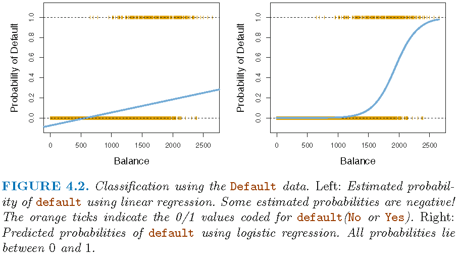
- Source: James et al. (2013, chaps. 4.3.1, 4.3.2, 4.3.4)
3.3 Logistic model: Compas data
- Logistic regression (LR) models the probability that \(Y\) belongs to a particular category (0 or 1)
- Rather than modeling response \(Y\) directly
- COMPAS data: Model probability to recidivate (reoffend)
- Outcome \(y\): Recidivism
reoffend(0,1,0,0,1,1,...) - Various predictors \(x's\)
- age =
age - prior offenses =
priors_count
- age =
- Outcome \(y\): Recidivism
- Use LR to obtain predicted values \(\hat{y}\)
- Predicted values will range between 0 and 1 = probabilities
- Depend on input/features (e.g., age, prior offences)
- Convert predicted values (probabilities) to a binary variable
- e.g., predict individuals will recidivate (
reoffend = Yes) if Pr(reoffend=Yes|age) > 0.5 - Here we call this variable
y_hat_01
- e.g., predict individuals will recidivate (
- Source: James et al. (2013, chap. 4.3)
3.4 Logistic model: Estimation
- Estimate model in R: glm(y ~ x1 + x2, family = binomial, data = data_train)
fit <- glm(as.factor(reoffend) ~ age + priors_count,
           family = binomial,
           data = data)
cat(paste(capture.output(summary(fit))[6:10], collapse="\n"))
Deviance Residuals:
Min 1Q Median 3Q Max
-3.1883 -1.0648 -0.5597 1.0989 2.5664
Coefficients:- R output shows log odds: e.g., a one-unit increase in
ageis associated with an increase in the log odds ofreoffendby-0.05units - Difficult to interpret.. much easier to use predicted probabilities
3.5 Logistic model: Prediction
augment(): Predict values in R (orpredict())- Once coefficients have been estimated, it is a simple matter to compute the probability of outcome for values of our predictors (James et al. 2013, 134)
augment(fit, newdata = ..., type.predict = "response")5: Predict probability for each unit- Use argument
type.predict="response"to output probabilities of form \(P(Y=1|X)\) (as opposed to other information such as the logit) - Use argument
newdata = ...to obtain predictions for new data
augment(fit, newdata = data_predict, type = "response"): Predict probability setting values for particular Xs (contained indata_predict)
data_new = data.frame(age = c(20, 20, 40, 40),
                          priors_count = c(0, 2, 0, 2))
data_new <- augment(fit, newdata = data_new, type.predict = "response")
data_new
# A tibble: 4 × 3
age priors_count .fitted
<dbl> <dbl> <dbl>
1 20 0 0.517
2 20 2 0.600
3 40 0 0.290
4 40 2 0.364- Q: How would you interpret these values?
- Source: James et al. (2013, chaps. 4.3.3, 4.6.2)
4 Classification (logistic model): Accuracy
- See James et al. (2013, Ch. 4.4.3)
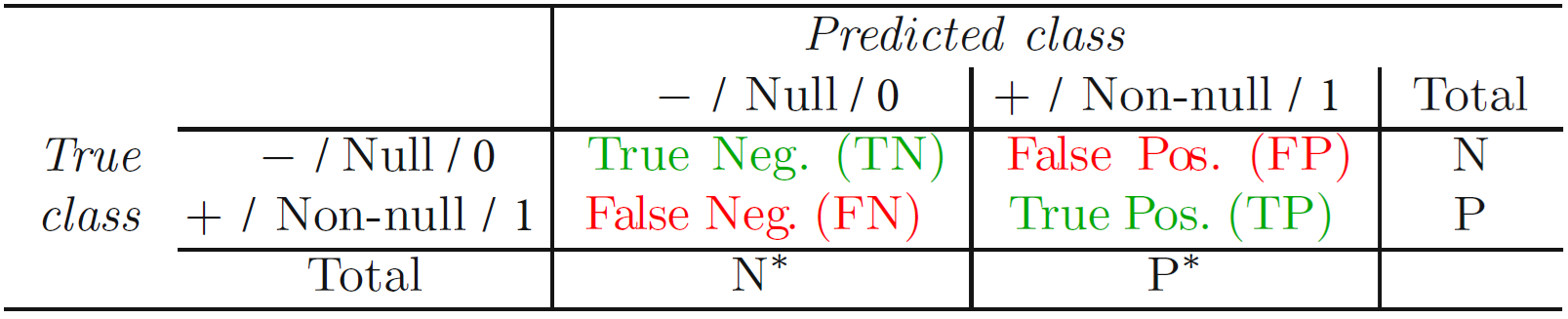
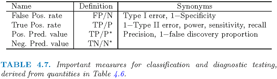
4.1 True/false negatives/positives
- Q: The tables in Figure 2 and Figure 3 illustrate how to calculate different accuracy metrics. Assuming the outcome is cancer (1 = yes, 0 = no), how could we interpret the different cells?
4.2 Exercise: Accuracy measures
- Global performance metrics:
- Accuracy (= correct classification rate): \(\frac{TP+TN}{TP+FP+TN+FN}\) (Error Rate= 1 − Accuracy)
- No Information rate6
- Row / column performance metrics:
| 0 | 1 | ||
| 0 | 80 (TN) | 10 (FP) | 90 (N) |
| 1 | 5 (FN) | 5 (TP) | 10 (P) |
| 85 (N*) | 15 (P*) | 100 (total) |
More…
- Precision
- Focus: How many of the predicted positive results are truly positive?
- Interpretation: Precision is important when the cost of false positives is high, for example, in spam email detection, where you want to avoid marking a legitimate email as spam.
- Recall
- Focus: How many of the actual positive cases are correctly identified?
- Interpretation: Recall is critical when missing a true positive has significant consequences, such as in medical diagnostics where you don’t want to miss a disease diagnosis.
- Specificity
- Focus: How many of the actual negative cases are correctly identified?
- Interpretation: Specificity matters when it is crucial to correctly identify negative cases, such as in a test where false alarms are costly or burdensome, like unnecessary medical tests.
- …there are various other measures!
4.3 F1-score
- F1-Score as further popular measure
- \(F1 = 2 \times \frac{precision \times recall}{precision + recall}\)
- Highest possible value of an F-score is 1.0, indicating perfect precision and recall, and the lowest possible value is 0, if either precision or recall are zero
- Why?
- F1-score combines both precision and recall into single score
- Precision measures accuracy of positive predictions; Recall measures how many actual positive instances were identified
- Useful when caring about both reducing false positives (high precision) and false negatives (high recall)
- Handles class imbalance better: considers both false positives and false negatives, providing a better sense of model’s performance with respect to the minority class
- Provides single metric for comparison
- F1-score combines both precision and recall into single score
4.4 Exercise: recidivism
- Take our recidivism example where reoffend = recidivate = 1 = positive and not reoffend = not recidivate = 0 and discuss the table in Figure 2 using this example.
- Take our recidivism example and discuss the different definitions (Column 2) in the Table in Figure 3. Explain what precision and recall would be in that case.
Answer
Precision \((TP/P^{*})\): \(\frac{\text{# of prisoners that reoffend AND are predicted to reoffend (true positives TP)}}{\text{# of all prisoners predicted to reoffend}}\)
Recall \((TP/P)\): \(\frac{\text{# of prisoners that reoffend AND are predicted to reoffend (true positives TP)}}{\text{# of all prisoners that reoffend and SHOULD have been predicted to reoffend (the "trues" P)}}\)
4.5 Error rates and ROC curve (binary classification)
- See James et al. (2013, Ch. 4.4.3)
- The error rates are a function of the classification threshold
- If we lower the classification threshold (e.g., use a predicted probability of 0.3 to classify someone as reoffender) we classify more items as positive (e.g. predict them to reoffend), thus increasing both False Positives and True Positives
- See James et al. (2013), Fig 4.7, p. 147
- Goal: we want to know how error rates develop as a function of the classification threshold
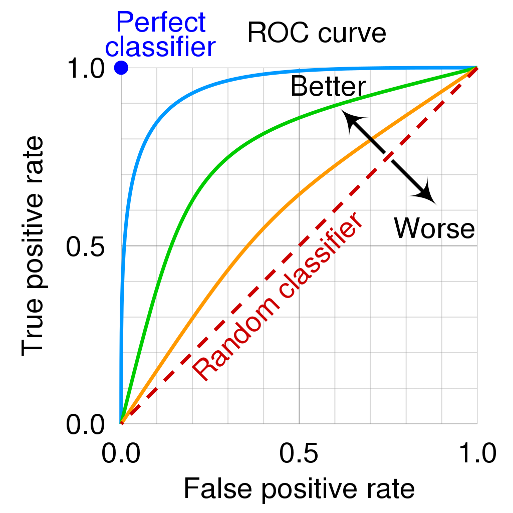
- The ROC curve is a popular graphic for simultaneously displaying the two types of errors (false positives, true positives rate) for all possible thresholds
- See James et al. (2013), Fig 4.8, p. 148 where \(1 - specificity\)\(= FP/N\)\(= \text{false positives rate (FPR)}\) and \(sensitivity\) \(= TP/P\)\(= \text{true positives rate (TPR)}\)
- The Area under the (ROC) curve (AUC) provides the overall performance of a classifier, summarized over all possible thresholds (James et al. 2013, 147)
- The maximum is 1, hence, values closer to it a preferable as shown in Figure 4 (maximize TRP, minimize FPR!)
Mnemonic bridge (Eselsbrücke) for sensitivity & specificity
Imagine you’re using a metal detector to search for gold (positive instances/cases). A sensitive detector beeps at almost every piece of gold, so it detects many (high true positive rate).
Imagine the metal detector is supposed to find only gold and not react to other trash (like bottles or aluminum foil). A specific detector focuses on the gold and ignores the rest.
- Sensitivity → Sniffer: Finds as many positives as possible, even if there are some false positives.
- Specificity → Selective: Focuses on correctly identifying negatives without false positives.
4.6 Weighting FPR and TPR differently (recidivism)
- Outcome: Recidivism where individual recidivates/reoffends (1) or not (0)
- False Positive (FP): Model predicts an individual will reoffend when they actually do not. This could lead to unnecessary interventions or harsher sentences for individuals.
- False Negative (FN): Model predicts an individual will not reoffend when they actually do. This could result in individuals who are at risk, being released without proper intervention, potentially leading to repeat offenses.
- Assign costs
- Cost of False Positive (FP): unnecessary prison time (costs for individual and society)
- Cost of False Negative (FN): repeat offenses (costs for society probably higher) (probably more important) → (weight FN more strongly)
- TPR (True positive rate) = 1- FNR (False negative rate)
- Pick threshold focusing on minimizing FN (ideally both FPR/FNR high!)
- Important: Probability threshold of classifying someone as 0/1 not shown in Figure 4
- We need to get it from the underlying calculations in Table 2
5 Lab: Classification using a logistic model
Learning outcomes/objective: Learn…
- …how to use trainingset and validation dataset for ML in R.
- …how to predict binary outcomes in R (using a simple logistic regression).
- …how to assess accuracy in R (logistic regression).
5.1 The data
Our lab is based on Lee, Du, and Guerzhoy (2020) and on James et al. (2013, chap. 4.6.2) with various modifications. We will be using the dataset at LINK that is described by Angwin et al. (2016). - It’s data based on the COMPAS risk assessment tools (RAT). RATs are increasingly being used to assess a criminal defendant’s probability of re-offending. While COMPAS seemingly uses a larger number of features/variables for the prediction, Dressel and Farid (2018) showed that a model that includes only a defendant’s sex, age, and number of priors (prior offences) can be used to arrive at predictions of equivalent quality.
Overview of Compas dataset variables
id: ID of prisoner, numericname: Name of prisoner, factorcompas_screening_date: Date of compass screening, datedecile_score: the decile of the COMPAS score, numericreoffend: whether somone reoffended/recidivated (=1) or not (=0), numericreoffend_factor: same but factor variableage: a continuous variable containing the age (in years) of the person, numericage_cat: age categorizedpriors_count: number of prior crimes committed, numericsex: gender with levels “Female” and “Male”, factorrace: race of the person, factorjuv_fel_count: number of juvenile felonies, numericjuv_misd_count: number of juvenile misdemeanors, numericjuv_other_count: number of prior juvenile convictions that are not considered either felonies or misdemeanors, numeric
We first import the data into R:
5.2 Inspecting the dataset
The variables were named quite well, so that they are often self-explanatory:
decile_scoreis the COMPAS scorereoffendwether someone reoffended (1 = recidividate = reoffend, 0 = NOT)racecontains the raceagecontains age.priors_countcontains the number of prior offenses- etc.
First we should make sure to really explore/unterstand our data. How many observations are there? How many different variables (features) are there? What is the scale of the outcome? What are the averages etc.? What kind of units are in your dataset?
[1] 7214[1] 14[1] 7214 14tibble [7,214 × 14] (S3: tbl_df/tbl/data.frame)
$ id : num [1:7214] 1 3 4 5 6 7 8 9 10 13 ...
$ name : Factor w/ 7158 levels "aajah herrington",..: 4922 4016 1989 4474 690 4597 2035 6345 2091 680 ...
$ compas_screening_date: Date[1:7214], format: "2013-08-14" "2013-01-27" ...
$ decile_score : num [1:7214] 1 3 4 8 1 1 6 4 1 3 ...
$ reoffend : num [1:7214] 0 1 1 0 0 0 1 NA 0 1 ...
$ reoffend_factor : Factor w/ 2 levels "no","yes": 1 2 2 1 1 1 2 NA 1 2 ...
$ age : num [1:7214] 69 34 24 23 43 44 41 43 39 21 ...
$ age_cat : Factor w/ 3 levels "25 - 45","Greater than 45",..: 2 1 3 3 1 1 1 1 1 3 ...
$ priors_count : num [1:7214] 0 0 4 1 2 0 14 3 0 1 ...
$ sex : Factor w/ 2 levels "Female","Male": 2 2 2 2 2 2 2 2 1 2 ...
$ race : Factor w/ 6 levels "African-American",..: 6 1 1 1 6 6 3 6 3 3 ...
$ juv_fel_count : num [1:7214] 0 0 0 0 0 0 0 0 0 0 ...
$ juv_misd_count : num [1:7214] 0 0 0 1 0 0 0 0 0 0 ...
$ juv_other_count : num [1:7214] 0 0 1 0 0 0 0 0 0 0 ...Also always inspect summary statistics for both numeric and categorical variables to get a better understanding of the data. Often such summary statistics will also reveal errors in the data.
Q: Does anything strike you as interesting the two tables below?
| Unique | Missing Pct. | Mean | SD | Min | Median | Max | Histogram | |
|---|---|---|---|---|---|---|---|---|
| id | 7214 | 0 | 5501.3 | 3175.7 | 1.0 | 5509.5 | 11001.0 |  |
| decile_score | 10 | 0 | 4.5 | 2.9 | 1.0 | 4.0 | 10.0 |  |
| reoffend | 3 | 9 | 0.5 | 0.5 | 0.0 | 0.0 | 1.0 |  |
| age | 65 | 0 | 34.8 | 11.9 | 18.0 | 31.0 | 96.0 |  |
| priors_count | 37 | 0 | 3.5 | 4.9 | 0.0 | 2.0 | 38.0 |  |
| juv_fel_count | 11 | 0 | 0.1 | 0.5 | 0.0 | 0.0 | 20.0 |  |
| juv_misd_count | 10 | 0 | 0.1 | 0.5 | 0.0 | 0.0 | 13.0 |  |
| juv_other_count | 10 | 0 | 0.1 | 0.5 | 0.0 | 0.0 | 17.0 |  |
| N | % | ||
|---|---|---|---|
| reoffend_factor | no | 3422 | 47.4 |
| yes | 3178 | 44.1 | |
| age_cat | 25 - 45 | 4109 | 57.0 |
| Greater than 45 | 1576 | 21.8 | |
| Less than 25 | 1529 | 21.2 | |
| sex | Female | 1395 | 19.3 |
| Male | 5819 | 80.7 | |
| race | African-American | 3696 | 51.2 |
| Asian | 32 | 0.4 | |
| Caucasian | 2454 | 34.0 | |
| Hispanic | 637 | 8.8 | |
| Native American | 18 | 0.2 | |
| Other | 377 | 5.2 |
The table() function is also useful to get an overview of variables. Use the argument useNA = "always" to display potential missings.
African-American Asian Caucasian Hispanic
3696 32 2454 637
Native American Other <NA>
18 377 0
no yes
0 3422 0
1 0 3178
1 2 3 4 5 6 7 8 9 10
1440 941 747 769 681 641 592 512 508 383 Finally, there are some helpful functions to explore missing data included in the naniar package. Can you decode those graphs? What do they show? (for publications the design would need to be improved)
5.3 Exploring potential predictors
A correlation matrix can give us first hints regarding important predictors.
- Q: Can we identify anything interesting?
5.4 Building a first logistic ML model
Below we estimate a simple logistic regression machine learning model only using one split into training and test data. To start, we check whether there are any missings on our outcome variable reoffend_factor (we use the factor version of our outcome variable). We extract the subset of individuals for whom our outcome reoffend_factor is missing, store them data_missing_outcome and delete those individuals from the actual dataset data.
# Extract data with missing outcome
data_missing_outcome <- data %>% filter(is.na(reoffend_factor))
dim(data_missing_outcome)[1] 614 14# Omit individuals with missing outcome from data
data <- data %>% drop_na(reoffend_factor) # ?drop_na
dim(data)[1] 6600 14
Then we split the data into training and test data.
# Split the data into training and test data
data_split <- initial_split(data, prop = 0.80)
data_split # Inspect<Training/Testing/Total>
<5280/1320/6600># Extract the two datasets
data_train <- training(data_split)
data_test <- testing(data_split) # Do not touch until the end!
dim(data_train)[1] 5280 14[1] 1320 14
Subsequently, we estimate our linear model based on the training data. Below we just use 1 predictor:
# Fit the model
fit1 <- logistic_reg() %>% # logistic model
set_engine("glm") %>% # define lm package/function
set_mode("classification") %>%# define mode
fit(reoffend_factor ~ age, # fit the model
data = data_train) # based on training data
fit1 # Class model output with summary(fit1$fit)parsnip model object
Call: stats::glm(formula = reoffend_factor ~ age, family = stats::binomial,
data = data)
Coefficients:
(Intercept) age
1.16380 -0.03548
Degrees of Freedom: 5279 Total (i.e. Null); 5278 Residual
Null Deviance: 7313
Residual Deviance: 7091 AIC: 7095# A tibble: 2 × 5
term estimate std.error statistic p.value
<chr> <dbl> <dbl> <dbl> <dbl>
1 (Intercept) 1.16 0.0891 13.1 5.12e-39
2 age -0.0355 0.00246 -14.4 2.95e-47
Then, we predict our outcome in the training data and evaluate the accuracy in the training data.
- Q: How can we interpret the accuracy metrics? Are we happy?11
# Training data: Add predictions
data_train %>%
augment(x = fit1, type.predict = "response") %>%
select(reoffend_factor, age, .pred_class, .pred_no, .pred_yes) %>%
head()# A tibble: 6 × 5
reoffend_factor age .pred_class .pred_no .pred_yes
<fct> <dbl> <fct> <dbl> <dbl>
1 yes 33 no 0.502 0.498
2 no 40 no 0.564 0.436
3 no 30 yes 0.475 0.525
4 no 24 yes 0.423 0.577
5 yes 24 yes 0.423 0.577
6 yes 32 yes 0.493 0.507# Cross-classification table (Columns = Truth, Rows = Predicted)
data_train %>%
augment(x = fit1, type.predict = "response") %>%
conf_mat(truth = reoffend_factor, estimate = .pred_class) Truth
Prediction no yes
no 1523 969
yes 1208 1580# Training data: Metrics
data_train %>%
augment(x = fit1, type.predict = "response") %>%
metrics(truth = reoffend_factor, estimate = .pred_class)# A tibble: 2 × 3
.metric .estimator .estimate
<chr> <chr> <dbl>
1 accuracy binary 0.588
2 kap binary 0.177
Finally, we can also predict data for the test data and evaluate the accuracy in the test data.
# Test data: Add predictions
data_test %>%
augment(x = fit1, type.predict = "response") %>%
select(reoffend_factor, age, .pred_class, .pred_no, .pred_yes) %>%
head()# A tibble: 6 × 5
reoffend_factor age .pred_class .pred_no .pred_yes
<fct> <dbl> <fct> <dbl> <dbl>
1 no 27 yes 0.449 0.551
2 yes 23 yes 0.414 0.586
3 no 41 no 0.572 0.428
4 yes 27 yes 0.449 0.551
5 no 43 no 0.590 0.410
6 yes 30 yes 0.475 0.525# Cross-classification table (Columns = Truth, Rows = Predicted)
data_test %>%
augment(x = fit1, type.predict = "response") %>%
conf_mat(truth = reoffend_factor, estimate = .pred_class) Truth
Prediction no yes
no 361 234
yes 330 395# Test data: Metrics
data_test %>%
augment(x = fit1, type.predict = "response") %>%
metrics(truth = reoffend_factor, estimate = .pred_class)# A tibble: 2 × 3
.metric .estimator .estimate
<chr> <chr> <dbl>
1 accuracy binary 0.573
2 kap binary 0.149Possible reasons if accuracy is higher on test data than training data:
Observing higher test accuracy may be due to:
- Bad training accuracy: Already bad accuracy in training data is easy to beat.
- Small Dataset: Test set may contain easier examples due to small dataset size.
- Overfitting to Test Data: Repeated tweaking against the same test set can lead to overfitting.
- Data Leakage: Information from the test set influencing the model during training.
- Strong Regularization: Techniques like dropout can make the model generalize better but underperform on training data.
- Evaluation Methodology: The splitting method can affect results, e.g., stratified splits.
- Random Variation: Small test sets can lead to non-representative results.
- Improper Training: Inadequate training epochs or improper learning rates.
5.4.1 ROC-curve
Below code to visualize the ROC-curve. The function roc_curve() calculates the data for the ROC curve.
# Calculate data for ROC curve - threshold, specificity, sensitivity
data_test %>%
augment(x = fit1, type.predict = "response") %>%
roc_curve(truth = reoffend_factor,
.pred_yes,
event_level = "second") %>%
head() %>% kable()| .threshold | specificity | sensitivity |
|---|---|---|
| -Inf | 0.0000000 | 1.0000000 |
| 0.1724511 | 0.0000000 | 1.0000000 |
| 0.1992575 | 0.0014472 | 1.0000000 |
| 0.2049793 | 0.0028944 | 1.0000000 |
| 0.2167862 | 0.0043415 | 1.0000000 |
| 0.2228713 | 0.0086831 | 0.9952305 |
We can then visualize the curve in Figure 5 is using autoplot(). Since it’s a ggplot we can make change labels etc. with +. Subsequently, we can use roc_auc() to calculate the area under the curve. Important (?roc_curve): Here we pick the 1s, i.e., recidivating as the “event” or “positive” result.12
# Calculate data for ROC curve and visualize
data_test %>%
augment(x = fit1, type.predict = "response") %>%
roc_curve(truth = reoffend_factor,
.pred_yes,
event_level = "second") %>% # Default: Uses first class (=0=no)
autoplot() +
xlab("False Positive Rate (FPR = FP/N = FP/(FP + TN), 1 - specificity)") +
ylab("True Positive Rate (TPR= TP/(TP + FN), sensitivity, recall)")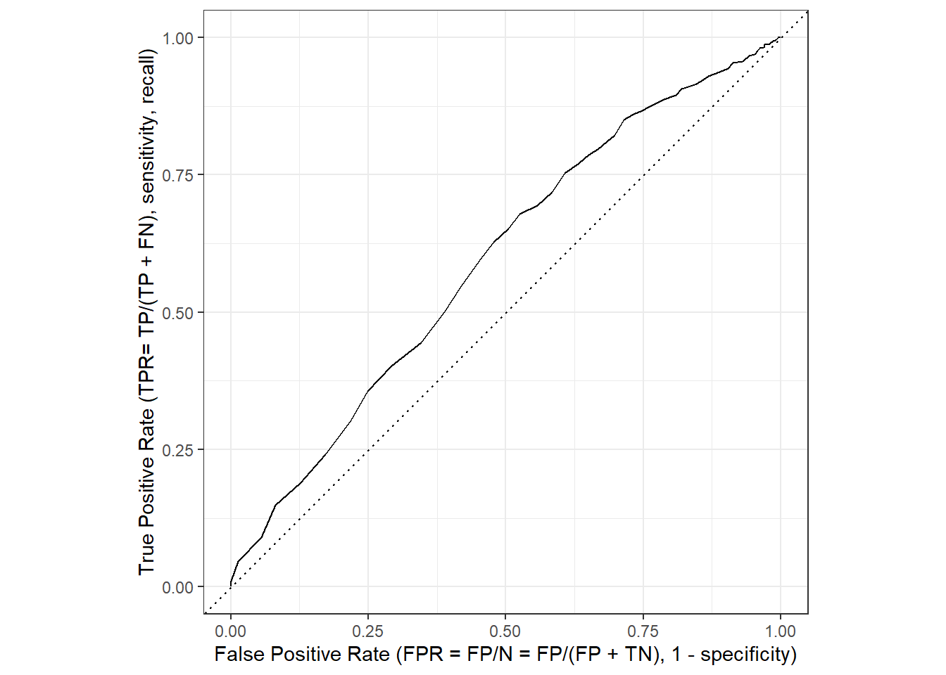
The area under the curve can be calculate with roc_auc().
# Calculate are under the curve
data_test %>%
augment(x = fit1, type.predict = "response") %>%
roc_auc(truth = reoffend_factor,
.pred_yes,
event_level = "second")# A tibble: 1 × 3
.metric .estimator .estimate
<chr> <chr> <dbl>
1 roc_auc binary 0.594
Importantly, the ROC curve does not provide information on how FPR and TPR change as a function of the threshold. In Figure 6 we visualize both precision and recall (TPR) as a function of the threshold. The pr_curve() function can be used to calculate the corresponding values and we could also change it to FPR vs. TPR.
library(ggplot2)
library(dplyr)
data_test %>%
augment(x = fit1, type.predict = "response") %>%
pr_curve(truth = reoffend_factor,
.pred_yes,
event_level = "second") %>%
pivot_longer(cols = c("recall", "precision"),
names_to = "measure",
values_to = "value") %>%
mutate(measure = recode(measure,
"recall" = "Recall (= True pos. rate = TP/P = sensitivity)",
"precision" = "Precision (= Pos. pred. value = TP/P*)")) %>%
ggplot(aes(x = .threshold,
y = value,
color = measure)) +
geom_line() +
xlab("Threshold value") +
ylab("Value of measure") +
theme_bw()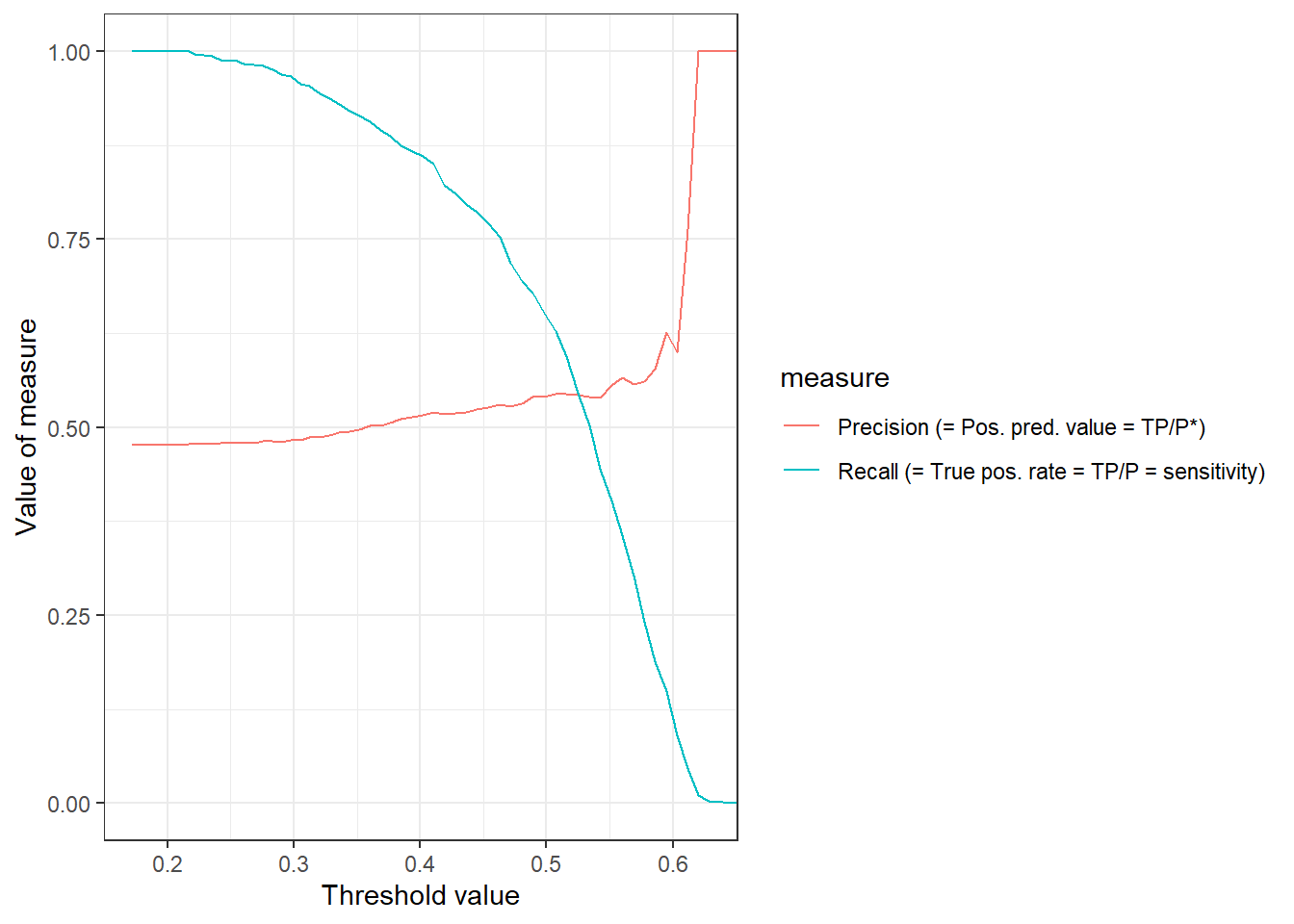
5.4.2 Predict unseen data
If we are happy with the accuracy in the test data we could then use our model to predict the outcomes for those individuals for which we did not observe the outcome which are stored in data_missing.
# Missing outcome data predictions
data_missing_outcome <- data_missing_outcome %>%
augment(x = fit1, type.predict = "response")
data_missing_outcome %>%
select(reoffend_factor, age, .pred_class, .pred_no, .pred_yes) %>%
head()# A tibble: 6 × 5
reoffend_factor age .pred_class .pred_no .pred_yes
<fct> <dbl> <fct> <dbl> <dbl>
1 <NA> 43 no 0.590 0.410
2 <NA> 31 yes 0.484 0.516
3 <NA> 21 yes 0.397 0.603
4 <NA> 32 yes 0.493 0.507
5 <NA> 30 yes 0.475 0.525
6 <NA> 21 yes 0.397 0.6035.4.3 Visualizing predictions
It is often insightful to visualize a MLM’s predictions, e.g., exploring whether our predictions are better or worse for certain population subsets (e.g., the young). In other words, whether the model works better/worse across groups. Below we take data_test from above (which includes the predictions) and calculate the errors and the absolute errors.
data_test %>%
augment(x = fit1, type.predict = "response") %>%
select(reoffend_factor, .pred_class, .pred_no, .pred_yes, age, sex, race, priors_count)# A tibble: 1,320 × 8
reoffend_factor .pred_class .pred_no .pred_yes age sex race priors_count
<fct> <fct> <dbl> <dbl> <dbl> <fct> <fct> <dbl>
1 no yes 0.449 0.551 27 Male Cauc… 0
2 yes yes 0.414 0.586 23 Male Afri… 3
3 no no 0.572 0.428 41 Male Afri… 0
4 yes yes 0.449 0.551 27 Male Cauc… 0
5 no no 0.590 0.410 43 Male Cauc… 1
6 yes yes 0.475 0.525 30 Male Cauc… 9
7 no yes 0.440 0.560 26 Male Cauc… 6
8 no yes 0.466 0.534 29 Male Cauc… 0
9 yes yes 0.466 0.534 29 Male Afri… 0
10 yes yes 0.431 0.569 25 Male Cauc… 9
# ℹ 1,310 more rowsFigure 7 visualizes the variation of the predicted probabilities. What can we see?
# Histogram of the predicted probabilities
data_test %>%
augment(x = fit1, type.predict = "response") %>%
ggplot(aes(x = .pred_yes)) +
geom_histogram() +
xlim(0,1)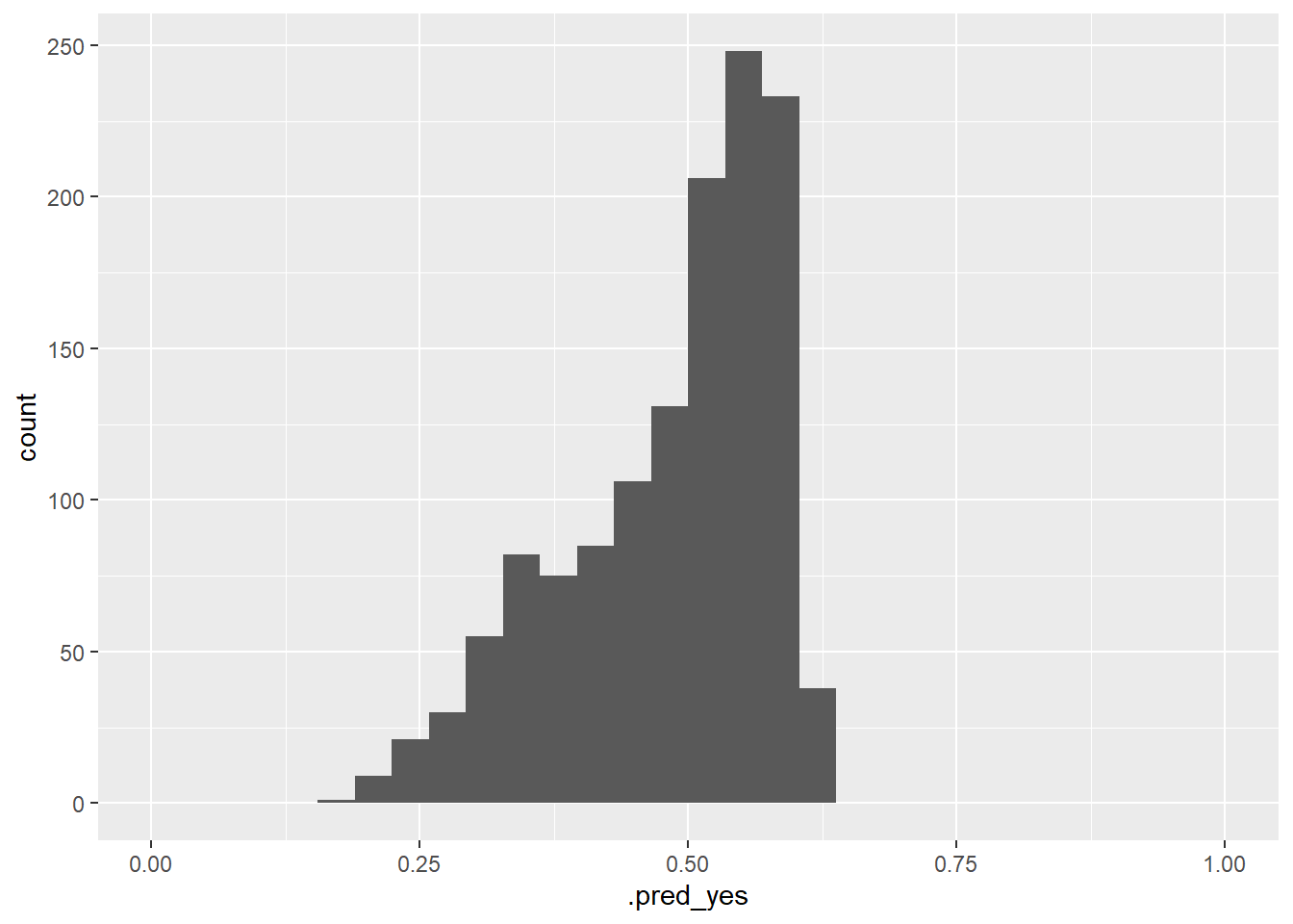
Figure 8 visualizes the variation of the predicted probabilities across groups. What can we see?
# Histogram of the predicted probabilities across groups
data_test %>%
augment(x = fit1, type.predict = "response") %>%
ggplot(aes(x = .pred_yes)) +
geom_histogram() +
facet_wrap(~race) +
xlim(0,1)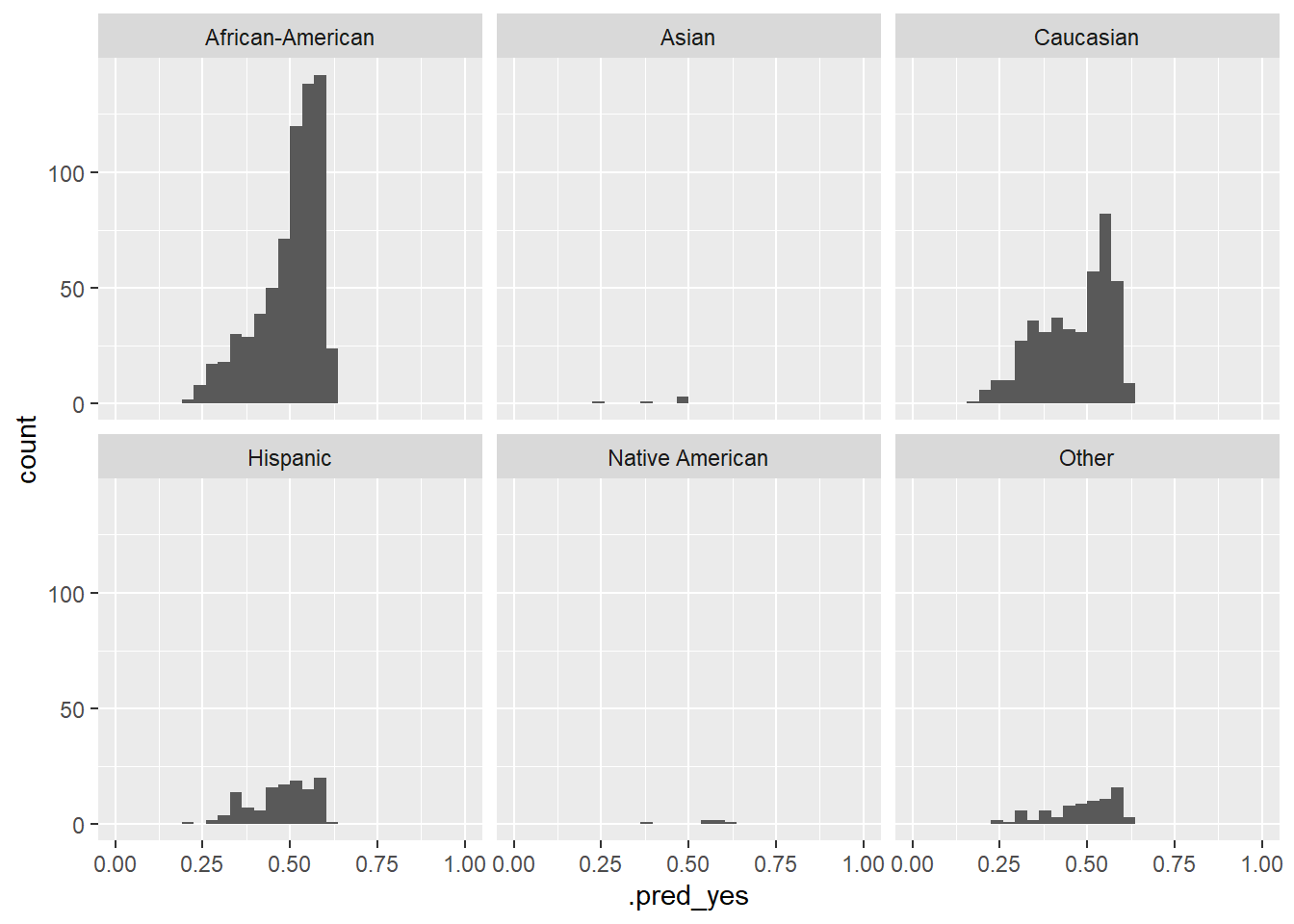
In Figure 9 we visualize the predicted probability of reoffending as a function of features after discretizing and factorizing some variables. Importantly, the ML model is only based on one of those variables namely age, hence, why the predictions do not vary that strongly with the other variables.
Q: What can we observe? What problem does that point to?
# Visualize errors and predictors
library(patchwork)
library(ggplot2)
data_plot <- data_test %>%
augment(x = fit1, type.predict = "response") %>%
select(.pred_yes, age, sex, race, priors_count) %>%
mutate(age = cut_interval(age, 8),
priors_count = as.factor(priors_count))
p1 <- ggplot(data = data_plot, aes(y = .pred_yes, x = sex)) +
geom_boxplot()
p2 <- ggplot(data = data_plot, aes(y = .pred_yes, x = age)) +
geom_boxplot() +
theme(axis.text.x = element_text(angle = 30, hjust = 1))
p3 <- ggplot(data = data_plot, aes(y = .pred_yes, x = race)) +
geom_boxplot() +
theme(axis.text.x = element_text(angle = 30, hjust = 1))
p4 <- ggplot(data = data_plot, aes(y = .pred_yes, x = priors_count)) +
geom_boxplot() +
theme(axis.text.x = element_text(angle = 30, hjust = 1))
p1 + p2 + p3 + p4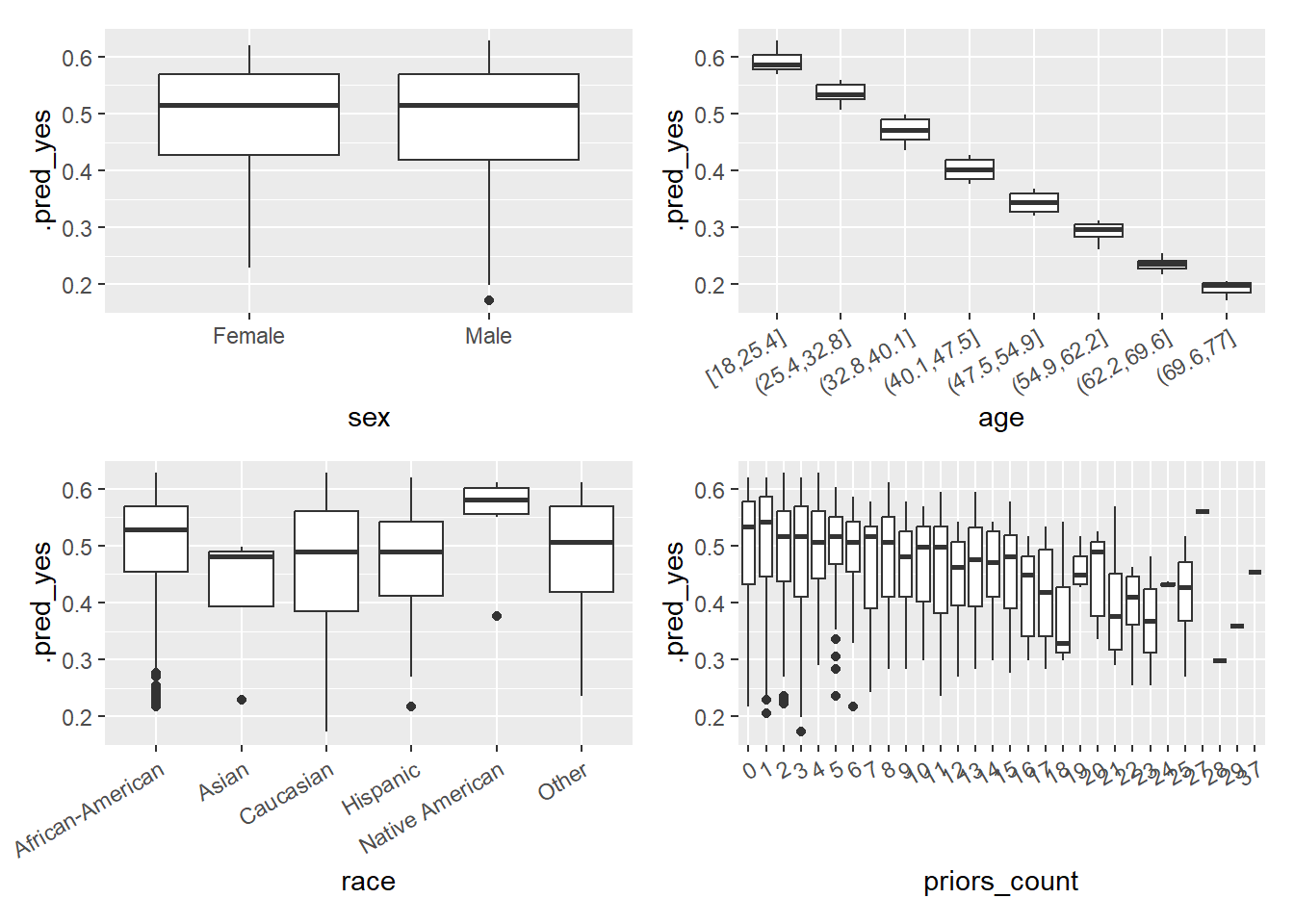
5.5 Altering the threshold
We can also explore how changing the threshold influences the accuracy overall and for the different ethnic groups. Below we generate a new predicted outcome variable .pred_class_thrshld that is based on picking different threshold using .pred_yes to classify someone as reoffender (= 1). Subsequently, we can use this new predicted outcome to calculate accuracy metrics.
# Make predictions & calculate accuracy
# picking different thresholds
data_test %>%
augment(x = fit1, type.predict = "response") %>%
mutate(.pred_class_thrshld = factor(ifelse(.pred_yes > 0.53, "yes", "no"),
levels = c("no", "yes"))) %>%
metrics(truth = reoffend_factor, estimate = .pred_class_thrshld)# A tibble: 2 × 3
.metric .estimator .estimate
<chr> <chr> <dbl>
1 accuracy binary 0.559
2 kap binary 0.113I just discovered the probably package (link) which has functions (e.g., threshold_perf()) to calculate accuracy metrics for different threshold. It’s probably worth it to check that out!
5.6 Exercise: Enhance simple logistic model
- Use the code below to load the data.
- In the next chunk you find the code we used above to built our first predictive model for our outcome
reoffend_factor. Please use the code and add further predictors to the model. Can you find a model with better accuracy picking further predictors?
# Extract data with missing outcome
data_missing_outcome <- data %>% filter(is.na(reoffend_factor))
dim(data_missing_outcome)
# Omit individuals with missing outcome from data
data <- data %>% drop_na(reoffend_factor) # ?drop_na
dim(data)
# Split the data into training and test data
data_split <- initial_split(data, prop = 0.80)
data_split # Inspect
# Extract the two datasets
data_train <- training(data_split)
data_test <- testing(data_split) # Do not touch until the end!
# Fit the model
fit1 <- logistic_reg() %>% # logistic model
set_engine("glm") %>% # define lm package/function
set_mode("classification") %>%# define mode
fit(reoffend_factor ~ age, # fit the model
data = data_train) # based on training data
fit1
# Training data: Add predictions
data_train %>%
augment(x = fit1, type.predict = "response") %>%
select(reoffend_factor, age, .pred_class, .pred_no, .pred_yes) %>%
head()
# Cross-classification table (Columns = Truth, Rows = Predicted)
data_train %>%
augment(x = fit1, type.predict = "response") %>%
conf_mat(truth = reoffend_factor, estimate = .pred_class)
# Training data: Metrics
data_train %>%
augment(x = fit1, type.predict = "response") %>%
metrics(truth = reoffend_factor, estimate = .pred_class)
# Test data: Add predictions
data_test %>%
augment(x = fit1, type.predict = "response") %>%
select(reoffend_factor, age, .pred_class, .pred_no, .pred_yes) %>%
head()
# Cross-classification table (Columns = Truth, Rows = Predicted)
data_test %>%
augment(x = fit1, type.predict = "response") %>%
conf_mat(truth = reoffend_factor, estimate = .pred_class)
# Test data: Metrics
data_test %>%
augment(x = fit1, type.predict = "response") %>%
metrics(truth = reoffend_factor, estimate = .pred_class)6 Homework/Exercise:
Above we used a logistic regression model to predict recidivism. In principle, we could also use a linear probability model, i.e., estimate a linear regression and convert the predicted probabilities to a predicted binary outcome variable later on.
- What might be a problem when we use a linear probability model to obtain predictions (see James et al. (2013), Figure, 4.2, p. 131)?
- Please use the code above (see next section below) but now change the model to a linear probability model using the same variables. How is the accuracy of the lp-model as compared to the logistic model? Did you expect that?
- Tipps
- The linear probability model is defined through
linear_reg() %>% set_engine('lm') %>% set_mode('regression') - The linear probability model provides a predicted probability that needs to be converted to a binary class variable at the end.
- The linear probability model requires a numeric outcome, i.e., use
reoffendas outcome and only convertreoffendto a factor at the end (as well as the predicted class).
- The linear probability model is defined through
Solution
# Extract data with missing outcome
data_missing_outcome <- data %>% filter(is.na(reoffend))
dim(data_missing_outcome)
# Omit individuals with missing outcome from data
data <- data %>% drop_na(reoffend) # ?drop_na
dim(data)
# Split the data into training and test data
data_split <- initial_split(data, prop = 0.80)
data_split # Inspect
# Extract the two datasets
data_train <- training(data_split)
data_test <- testing(data_split) # Do not touch until the end!
# Fit the model
fit1 <- linear_reg() %>% # logistic model
set_engine("lm") %>% # define lm package/function
set_mode("regression") %>%# define mode
fit(reoffend ~ age, # fit the model
data = data_train) # based on training data
fit1
# Training data: Add predictions
data_train <- augment(x = fit1, data_train) %>%
mutate(.pred_class = as.factor(ifelse(.pred>=0.5, 1, 0)),
reoffend = factor(reoffend))
head(data_train %>%
select(reoffend, reoffend_factor, age, .pred, .resid, .pred_class))
# Training data: Metrics
data_train %>%
metrics(truth = reoffend, estimate = .pred_class)
# Test data: Add predictions
data_test <- augment(x = fit1, data_test) %>%
mutate(.pred_class = as.factor(ifelse(.pred>=0.5, 1, 0)),
reoffend = factor(reoffend))
head(data_test %>%
select(reoffend, reoffend_factor, age, .pred, .resid, .pred_class))
# Test data: Metrics
data_test %>%
metrics(truth = reoffend, estimate = .pred_class) 6.1 All the code
# namer::unname_chunks("03_01_predictive_models.qmd")
# namer::name_chunks("03_01_predictive_models.qmd")
options(scipen=99999)
#| echo: false
library(tidyverse)
library(lemon)
library(knitr)
library(kableExtra)
library(dplyr)
library(plotly)
library(randomNames)
library(stargazer)
library(gt)
library(tidymodels)
library(tidyverse)
set.seed(0)
load("www/data/data_compas.RData")
data_table <- data %>% select(id, name, compas_screening_date, reoffend,
reoffend_factor, age, priors_count) %>%
slice(1:10)
data_table %>%
kable(format = "html",
escape=FALSE,
align=c(rep("l", 1), "c", "c")) %>%
kable_styling(font_size = 16)
library(tidyverse)
set.seed(0)
load(file = "www/data/data_compas.Rdata")
# First 5000 observations as training data
data_train <- data[1:5000,]
fit <- glm(as.factor(reoffend) ~ age + priors_count,
family = binomial,
data = data)
cat(paste(capture.output(summary(fit))[6:10], collapse="\n"))
ggplot(data_train) + geom_smooth(aes(x = priors_count, y = y_hat)) + geom_point(aes(x = priors_count, y = reoffend)) + ylim(0,1)
data_new = data.frame(age = c(20, 20, 40, 40),
priors_count = c(0, 2, 0, 2))
data_new <- augment(fit, newdata = data_new, type.predict = "response")
data_new
# Visualize predicted values in plot
fit_linear <- lm(reoffend ~ age,
data = data_train)
data_train$y_hat_lm <- predict(fit_linear, type = "response")
ggplot(data = data_train, aes(x = age, y = reoffend)) +
geom_jitter(width = 0.1, height = 0.1, alpha = 0.1) +
geom_point(aes(x = age, y = y_hat), color = "red") +
geom_point(aes(x = age, y = y_hat_lm), color = "blue")
fit <- glm(as.factor(reoffend) ~ age,
family = binomial,
data = data_train)
fit2 <- lm(reoffend ~ age,
data = data_train)
data_train$y_hat <- predict(fit, type = "response")
data_train$y_hat2 <- predict(fit2, type = "response")
ggplot(data_train) +
geom_smooth(aes(x = priors_count, y = y_hat)) +
#geom_smooth(aes(x = priors_count, y = y_hat2)) +
geom_point(aes(x = priors_count, y = reoffend)) +
ylim(0,1)
x <- structure(c(540L, 255L, 224L, 424L),
dim = c(2L, 2L),
dimnames = structure(list(
c("0", "1"),
c("0", "1")),
names = c("", "")),
class = "table")
x <- cbind(x, rowSums(x))
x <- rbind(x, colSums(x))
x <- as.data.frame.matrix(x)
rownames(x)[3] <- "Total"
names(x)[3] <- "Total"
x <- x %>%
mutate(row_spanner = "True/actual values") %>%
mutate(category = rownames(.)) %>%
remove_rownames() %>%
select(category, row_spanner, everything())
confusion_matrix_reduced <- gt::gt(x,
#rownames_to_stub = TRUE,
rowname_col = "category",
groupname_col = "row_spanner") %>%
tab_spanner(
label = "Predicted values",
columns = c("0","1")
) |>
cols_width(everything() ~ px(120)) |>
tab_header(
title = md("Outcome recidivism:<br> 1 = reoffend, 0 = not reoffend"))
gtsave(data = confusion_matrix_reduced, filename = "confusion_matrix_reduced.png")
# Add names
x[1,3] <- paste0(x[1,3], " (TN)")
x[2,3] <- paste0(x[2,3], " (FN)")
x[1,4] <- paste0(x[1,4], " (FP)")
x[2,4] <- paste0(x[2,4], " (TP)")
x[3,3] <- paste0(x[3,3], " (N*)")
x[3,4] <- paste0(x[3,4], " (P*)")
x[1,5] <- paste0(x[1,5], " (N)")
x[2,5] <- paste0(x[2,5], " (P)")
confusion_matrix <- gt::gt(x,
#rownames_to_stub = TRUE,
rowname_col = "category",
groupname_col = "row_spanner") %>%
tab_spanner(
label = "Predicted values",
columns = c("0","1")
) |>
cols_width(everything() ~ px(120) ) |>
tab_header(
title = md("Outcome recidivism:<br> 1 = reoffend, 0 = not reoffend"))
confusion_matrix
gtsave(data = confusion_matrix, filename = "confusion_matrix.png")
# install.packages(pacman)
pacman::p_load(tidyverse,
tidymodels,
knitr,
kableExtra,
DataExplorer,
visdat,
naniar)
load(file = "www/data/data_compas.Rdata")
# install.packages(pacman)
pacman::p_load(tidyverse,
               tidymodels,
               knitr,
               kableExtra,
               DataExplorer,
               visdat,
               naniar)

rm(list=ls())
load(url(sprintf("https://docs.google.com/uc?id=%s&export=download",
                         "1gryEUVDd2qp9Gbgq8G0PDutK_YKKWWIk")))
nrow(data)
ncol(data)
dim(data)
str(data) # Better use glimpse()
# glimpse(data)
# skimr::skim(data)
library(modelsummary)
datasummary_skim(data, type = "numeric", output = "html")
datasummary_skim(data, type = "categorical", output = "html")
table(data$race, useNA = "always")
table(data$reoffend, data$reoffend_factor)
table(data$decile_score)
vis_miss(data)
gg_miss_upset(data, nsets = 2, nintersects = 10)
# Ideally, use higher number of nsets/nintersects
# with more screen space
plot_correlation(data %>% dplyr::select(reoffend, age,
                                        priors_count,sex,
                                        race,
                                        juv_fel_count),
                 cor_args = list("use" = "pairwise.complete.obs"))
# Extract data with missing outcome
  data_missing_outcome <- data %>% filter(is.na(reoffend_factor))
  dim(data_missing_outcome)
# Omit individuals with missing outcome from data
  data <- data %>% drop_na(reoffend_factor) # ?drop_na
  dim(data)
# Split the data into training and test data
  data_split <- initial_split(data, prop = 0.80)
  data_split # Inspect
# Extract the two datasets
  data_train <- training(data_split)
  data_test <- testing(data_split) # Do not touch until the end!
  dim(data_train)
dim(data_test)
# Fit the model
  fit1 <- logistic_reg() %>% # logistic model
        set_engine("glm") %>% # define lm package/function
        set_mode("classification") %>%# define mode
        fit(reoffend_factor ~ age, # fit the model
        data = data_train) # based on training data
  fit1 # Class model output with summary(fit1$fit)
tidy(fit1) # extract model coefficients/parameters
# Training data: Add predictions
data_train %>%
  augment(x = fit1, type.predict = "response") %>%
    select(reoffend_factor, age, .pred_class, .pred_no, .pred_yes) %>%
      head()
# Cross-classification table (Columns = Truth, Rows = Predicted)
data_train %>%
  augment(x = fit1, type.predict = "response") %>%
      conf_mat(truth = reoffend_factor, estimate = .pred_class)
# Training data: Metrics
data_train %>%
  augment(x = fit1, type.predict = "response") %>%
      metrics(truth = reoffend_factor, estimate = .pred_class)
# Test data: Add predictions
  data_test %>%
    augment(x = fit1, type.predict = "response") %>%
    select(reoffend_factor, age, .pred_class, .pred_no, .pred_yes) %>%
      head()
# Cross-classification table (Columns = Truth, Rows = Predicted)
  data_test %>%
    augment(x = fit1, type.predict = "response") %>%
      conf_mat(truth = reoffend_factor, estimate = .pred_class)
# Test data: Metrics
  data_test %>%
    augment(x = fit1, type.predict = "response") %>%
      metrics(truth = reoffend_factor, estimate = .pred_class)
# Calculate data for ROC curve - threshold, specificity, sensitivity
  data_test %>%
    augment(x = fit1, type.predict = "response") %>%
      roc_curve(truth = reoffend_factor,
            .pred_yes,
            event_level = "second") %>%
  head() %>% kable()
# Calculate are under the curve
  data_test %>%
    augment(x = fit1, type.predict = "response") %>%
      roc_auc(truth = reoffend_factor,
            .pred_yes,
            event_level = "second")
# Missing outcome data predictions
  data_missing_outcome <- data_missing_outcome %>%
                                augment(x = fit1, type.predict = "response")

  data_missing_outcome %>%
    select(reoffend_factor, age, .pred_class, .pred_no, .pred_yes) %>%
        head()
data_test %>%
    augment(x = fit1, type.predict = "response") %>%
        select(reoffend_factor, .pred_class, .pred_no, .pred_yes, age, sex, race, priors_count)
# Histogram of the predicted probabilities
data_test %>%
    augment(x = fit1, type.predict = "response") %>%
ggplot(aes(x = .pred_yes)) +
  geom_histogram() +
  xlim(0,1)
# Histogram of the predicted probabilities across groups
data_test %>%
    augment(x = fit1, type.predict = "response") %>%
    ggplot(aes(x = .pred_yes)) +
    geom_histogram() +
    facet_wrap(~race) +
    xlim(0,1)
# Visualize errors and predictors
library(patchwork)
library(ggplot2)
data_plot <- data_test %>%
    augment(x = fit1, type.predict = "response") %>%
  select(.pred_yes, age, sex, race, priors_count) %>%
  mutate(age = cut_interval(age, 8),
         priors_count = as.factor(priors_count))


p1 <- ggplot(data = data_plot, aes(y = .pred_yes, x = sex)) +
  geom_boxplot()
p2 <- ggplot(data = data_plot, aes(y = .pred_yes, x =  age)) +
  geom_boxplot() +
      theme(axis.text.x = element_text(angle = 30, hjust = 1))
p3 <- ggplot(data = data_plot, aes(y = .pred_yes, x = race)) +
      geom_boxplot() +
      theme(axis.text.x = element_text(angle = 30, hjust = 1))
p4 <- ggplot(data = data_plot, aes(y = .pred_yes, x = priors_count)) +
      geom_boxplot() +
      theme(axis.text.x = element_text(angle = 30, hjust = 1))
p1 + p2 + p3 + p4
# Make predictions & calculate accuracy
# picking different thresholds
  data_test %>%
      augment(x = fit1, type.predict = "response") %>%
  mutate(.pred_class_thrshld = factor(ifelse(.pred_yes > 0.53, "yes", "no"),
                                          levels = c("no", "yes"))) %>%
      metrics(truth = reoffend_factor, estimate = .pred_class_thrshld)
# install.packages(pacman)
pacman::p_load(tidyverse,
tidymodels,
knitr,
kableExtra,
DataExplorer,
naniar)
load(file = "www/data/data_compas.Rdata")
# install.packages(pacman)
pacman::p_load(tidyverse,
               tidymodels,
               knitr,
               kableExtra,
               DataExplorer,
               naniar)

rm(list=ls())
load(url(sprintf("https://docs.google.com/uc?id=%s&export=download",
                         "1gryEUVDd2qp9Gbgq8G0PDutK_YKKWWIk")))
# Extract data with missing outcome
  data_missing_outcome <- data %>% filter(is.na(reoffend_factor))
  dim(data_missing_outcome)

# Omit individuals with missing outcome from data
  data <- data %>% drop_na(reoffend_factor) # ?drop_na
  dim(data)

# Split the data into training and test data
  data_split <- initial_split(data, prop = 0.80)
  data_split # Inspect

# Extract the two datasets
  data_train <- training(data_split)
  data_test <- testing(data_split) # Do not touch until the end!


# Fit the model
  fit1 <- logistic_reg() %>% # logistic model
        set_engine("glm") %>% # define lm package/function
        set_mode("classification") %>%# define mode
        fit(reoffend_factor ~ age, # fit the model
        data = data_train) # based on training data
  fit1

# Training data: Add predictions
data_train %>%
  augment(x = fit1, type.predict = "response") %>%
    select(reoffend_factor, age, .pred_class, .pred_no, .pred_yes) %>%
      head()

# Cross-classification table (Columns = Truth, Rows = Predicted)
data_train %>%
  augment(x = fit1, type.predict = "response") %>%
      conf_mat(truth = reoffend_factor, estimate = .pred_class)

# Training data: Metrics
data_train %>%
  augment(x = fit1, type.predict = "response") %>%
      metrics(truth = reoffend_factor, estimate = .pred_class)


# Test data: Add predictions
  data_test %>%
    augment(x = fit1, type.predict = "response") %>%
    select(reoffend_factor, age, .pred_class, .pred_no, .pred_yes) %>%
      head()

# Cross-classification table (Columns = Truth, Rows = Predicted)
  data_test %>%
    augment(x = fit1, type.predict = "response") %>%
      conf_mat(truth = reoffend_factor, estimate = .pred_class)

# Test data: Metrics
  data_test %>%
    augment(x = fit1, type.predict = "response") %>%
      metrics(truth = reoffend_factor, estimate = .pred_class)
# install.packages(pacman)
pacman::p_load(tidyverse,
tidymodels,
knitr,
kableExtra,
DataExplorer,
visdat,
naniar)
load(file = "www/data/data_compas.Rdata")
# install.packages(pacman)
pacman::p_load(tidyverse,
               tidymodels,
               knitr,
               kableExtra,
               DataExplorer,
               visdat,
               naniar)

rm(list=ls())
load(url(sprintf("https://docs.google.com/uc?id=%s&export=download",
                         "1gryEUVDd2qp9Gbgq8G0PDutK_YKKWWIk")))
# Extract data with missing outcome
  data_missing_outcome <- data %>% filter(is.na(reoffend))
  dim(data_missing_outcome)

# Omit individuals with missing outcome from data
  data <- data %>% drop_na(reoffend) # ?drop_na
  dim(data)

# Split the data into training and test data
  data_split <- initial_split(data, prop = 0.80)
  data_split # Inspect

# Extract the two datasets
  data_train <- training(data_split)
  data_test <- testing(data_split) # Do not touch until the end!


# Fit the model
  fit1 <- linear_reg() %>% # logistic model
        set_engine("lm") %>% # define lm package/function
        set_mode("regression") %>%# define mode
        fit(reoffend ~ age, # fit the model
        data = data_train) # based on training data
  fit1

# Training data: Add predictions
  data_train <- augment(x = fit1, data_train) %>%
  mutate(.pred_class = as.factor(ifelse(.pred>=0.5, 1, 0)),
         reoffend = factor(reoffend))

  head(data_train %>%
      select(reoffend, reoffend_factor, age, .pred, .resid, .pred_class))

# Training data: Metrics
  data_train %>%
      metrics(truth = reoffend, estimate = .pred_class)


# Test data: Add predictions
  data_test <- augment(x = fit1, data_test) %>%
  mutate(.pred_class = as.factor(ifelse(.pred>=0.5, 1, 0)),
         reoffend = factor(reoffend))

  head(data_test %>%
      select(reoffend, reoffend_factor, age, .pred, .resid, .pred_class))

# Test data: Metrics
  data_test %>%
      metrics(truth = reoffend, estimate = .pred_class)
labs = knitr::all_labels()
labs = setdiff(labs, c("setup", "setup2", "homework-solution-hide", "get-labels", "load-data-1"))References
Angwin, Julia, Jeff Larson, Lauren Kirchner, and Surya Mattu. 2016. “Machine Bias.” https://www.propublica.org/article/machine-bias-risk-assessments-in-criminal-sentencing.
Dressel, Julia, and Hany Farid. 2018. “The Accuracy, Fairness, and Limits of Predicting Recidivism.” Science Advances 4 (1): eaao5580.
James, Gareth, Daniela Witten, Trevor Hastie, and Robert Tibshirani. 2013. An Introduction to Statistical Learning: With Applications in R. Springer.
Lee, Claire S, Jeremy Du, and Michael Guerzhoy. 2020. “Auditing the COMPAS Recidivism Risk Assessment Tool: Predictive Modelling and Algorithmic Fairness in CS1.” In Proceedings of the 2020 ACM Conference on Innovation and Technology in Computer Science Education, 535–36. Association for Computing Machinery.
Footnotes
The logistic function and the sigmoid function are often used interchangeably in practice because they describe the same mathematical form. Sigmoid is a general term for any function with an “S”-shaped curve. The logistic function is a specific type of sigmoid function.↩︎
The standard logistic regression function is given by: \(f(x) = \frac{1}{1 + e^{-y}}\) where \(y = \beta_0 + \beta_1x_1 + \beta_2x_2 + \dots + \beta_nx_n\).To rewrite the equation such that \(e\) appears in both the numerator and denominator, multiply both the numerator and denominator by \(e^{y}\): \(f(x) = \frac{1 \cdot e^{y}}{e^{y}(1 + e^{-y})}\). Since \(e^{y} \cdot e^{-y} = 1\), the denominator simplifies to: \(f(x) = \frac{e^{y}}{e^{y} + 1}\). The logistic regression function with \(e\) in both the numerator and denominator is: \(f(x) = \frac{e^{y}}{e^{y} + 1}\) where \(y = \beta_0 + \beta_1x_1 + \beta_2x_2 + \dots + \beta_nx_n\).↩︎
Here \(y = f(x)\) has been replaced with \(p(X)\).↩︎
In logistic regression, the “odds” represent the ratio of the probability of an event occurring to the probability of the event not occurring. They are used to quantify the likelihood of a certain outcome based on predictor variables. In logistic regression, the odds can take any non-negative value, from zero to infinity. A value of zero indicates the event will never occur, while larger values indicate a greater likelihood of the event occurring.↩︎
Alternatively use
predict(fit, newdata = NULL, type = "response").↩︎The No Information Rate (NIR) is the accuracy that could be achieved by always predicting the most frequent class in the dataset. If in a dataset 70% of the samples belong to class A (= populist tweets), the NIR would be 70%, since predicting class A for every sample would result in 70% accuracy.↩︎
# of true positive results (TP) divided by the # of all samples that should have been identified as positive (P = TP + FN). Example: # of patients that have cancer AND are predicted to have cancer (true positives TP) – divided by – # of all patients that have cancer (P) (and SHOULD have been predicted to have cancer)↩︎
# of true negative results (TN) divided by the # of all samples that should have been identified as negative (N = TN + FP). Example: # of patients that don’t have cancer AND are predicted to NOT have cancer (true negatives TN) – divided by – # of all patients that don’t have cancer (N) (and SHOULD have been predicted to NOT have cancer)↩︎
# of true positive (TP) results divided by the # of all positive results (P*= TP + FP), including those not identified correctly. Example: # of patients that have cancer AND are predicted to have cancer (true positives TP) – divided by – # of all patients predicted to have cancer (positives P*)↩︎
Accuracy = 85%; Sensitivity = 50%; Specificity = 88.89%; Precision = 33.33%↩︎
Kappa is a similar measure to accuracy, but is normalized by the accuracy that would be expected by chance alone and is very useful when one or more classes have large frequency distributions.↩︎
“There is no common convention on which factor level should automatically be considered the”event” or “positive” result when computing binary classification metrics. In yardstick, the default is to use the first level. To alter this, change the argument event_level to “second” to consider the last level of the factor the level of interest.” (see
?roc_curve)↩︎