| \(\text{Unit i} \quad\) | \(Name \quad\) | \(X1_{i}^{Age} \quad\) | \(X2_{i}^{Educ.} \quad\) | \(Y_{i}^{Lifesat.} \quad\) |
|---|---|---|---|---|
| 1 | Sofia | 29 | 1 | 3 |
| 2 | Sara | 30 | 2 | 2 |
| 3 | José | 28 | 0 | 5 |
| 4 | Yiwei | 27 | 2 | ? |
| 5 | Julia | 25 | 0 | 6 |
| 6 | Hans | 23 | 0 | ? |
| .. | .. | .. | .. | .. |
| 1000 | Hugo | 23 | 1 | 8 |
Further topics & summary & outlook
Chapter last updated: 10 Februar 2025
1 Using LLMs/foundationa models to built predictive models
1.1 Attention: Hallucination..
- Attention: Always cross-validate the information given by a LLM
- Why? Hallucination.. (see characterization statements on Wikipedia)
- “a tendency to invent facts in moments of uncertainty” (OpenAI, May 2023)
- “a model’s logical mistakes” (OpenAI, May 2023)
- fabricating information entirely, but behaving as if spouting facts (CNBC, May 2023)
- “making up information” (The Verge, February 2023)
- Why? Hallucination.. (see characterization statements on Wikipedia)
- Very good overview on Wikipedia
- Discussions in Zhang et al. (2023), Huang et al. (2023) and Metz (2023)
1.2 Avaible LLMs
- Closed-source
- ChatGPT X (OpenAI, ~Microsoft): https://chat.openai.com/
- Gemini (Google) https://gemini.google.com/
- Amazon Titan: https://aws.amazon.com/bedrock/titan/
- Open-source
- HuggingChat: https://huggingface.co/chat/
- Curated list of papers about large language models
- Top Open-Source LLMs for 2024 and Their Uses
1.3 Useful prompts
LLMs can be used to discuss theory underlying ML and generate code for ML
Data preparation & preprocessing
How do I need to prepare and preprocess the data if I want to built a Naive Bayes classifier?


What is particular in data preparation for Naive Bayes that is not necessary for other machine learning models?


How should I ideally preprocess the data that I feed into a Naive Bayes classifier?
I want to build a Naive Bayes Classifier. Please outline the preprocessing steps that you would recommend and provide tidymodels recipe code that includes those step.
Please write the code into a single recipe.- Understanding & comparing models
What is the difference between a logistic regression model and naive bayes in the machine learning context?


Which machine learning models that we can use for classification have a problem with class imbalance?- Understanding code
Please explain the hyperparamters in this model:

xgb_spec <- boost_tree(
  trees = 1000,
  tree_depth = tune(), min_n = tune(),
  loss_reduction = tune(),                     ## first three: model complexity
  sample_size = tune(), mtry = tune(),         ## randomness
  learn_rate = tune()                          ## step size
) %>%
  set_engine("xgboost") %>%
  set_mode("classification")
Followed by:
Please further explain the learn_rate:
- Data management: Below copy descriptions from ESS codebook and create better variable names.
Please provide dplyr code to rename the following variables and give them better names (lowercaps). Below is the codebook:

pdwrk - Doing last 7 days: paid work
edctn - Doing last 7 days: education
uempla - Doing last 7 days: unemployed, actively looking for job
uempli - Doing last 7 days: unemployed, not actively looking for job
dsbld - Doing last 7 days: permanently sick or disabled
rtrd - Doing last 7 days: retired
cmsrv - Doing last 7 days: community or military service
hswrk - Doing last 7 days: housework, looking after children, others
dngoth - Doing last 7 days: other
dngref - Doing last 7 days: refusal
dngdk - Doing last 7 days: don't know
dngna - Doing last 7 days: no answer
2 Classical statistics vs. machine learning (skip!)
Questions/Learning outcomes: Understand difference between classic statistics and machine learning.
2.1 Cultures and goals
- Two cultures of statistical analysis (Breiman 2001; Molina and Garip 2019, 29)
- Data modeling vs. algorithmic modeling (Breiman 2001)
- \(\approx\) generative modelling vs. algorithmic modeling (Donoho 2017)
- Data modeling vs. algorithmic modeling (Breiman 2001)
- Generative modeling (classical statistics, Objective: Inference/explanation)
- Goal: understand how an outcome is related to inputs
- Analyst proposes a stochastic model that could have generated the data, and estimates the parameters of the model from the data
- Leads to simple and interpretable models BUT often ignores model uncertainty and out-of-sample performance
- Predictive modeling (Objective: Prediction)
- Goal: prediction, i.e., forecast the outcome for unseen (Q: ?) or future observations
- Analyst treats underlying generative model for data as unknown and primarily considers the predictive accuracy of alternative models on new data
- Leads to complex models that perform well out of sample BUT can produce black-box results that offer little insight on the mechanism linking the inputs to the output (but Interpretable ML)
- Example: Predicting/explaining unemployment with a linear regression model
- See also James et al. (2013, Ch. 2.1.1)
2.2 Machine learning as programming (!) paradigm
- ML reflects a different programming paradigm (Chollet and Allaire 2018, chap. 1.1.2)
- Machine learning arises from this question: could a computer […] learn on its own how to perform a specified task? […] Rather than programmers crafting data-processing rules by hand, could a computer automatically learn these rules by looking at data?
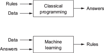
- Classical programming (paradigm of symbolic AI)
- Humans input rules (a program) and data to be processed according to these rules, and out come answers
- Machine learning paradigm
- Humans input data + answers expected from the data, and out come the rules [these rules can then be applied to new data]
- ML system is trained rather than explicitly programmed
- Trained: Presented with many examples relevant to a task → finds statistical structure in these examples &rarr allows system to come up with rules for automating the task (remember Alpha Go)
- Role of math
- While related to math. statistics, ML tends to deal with large, complex datasets (e.g., millions of images, each consisting of thousands of pixels)
- As a result ML (especially deep learning) exhibits comparatively little mathematical theory and is engineering oriented (ideas proven more often empirically than mathematically) (Chollet and Allaire 2018, chap. 1.1.2)
3 Timeline of statistical learning
- Source: James et al. (2013, 6–7)
- Beginning of the 19th century: Legendre and Gauss - method of least squares
- Earliest form of linear regression (Astronomy)
- 1936: Fisher - Linear Discriminant Analysis
- 1940s: various authors - Logistic Regression
- 1970: Nelder and Wedderburn - Generalized Linear Models (GLM) of which linear and logistic regression are special cases
- By end of the 1970s: Many more techniques available but almost exclusively linear methods
- Fitting non-linear relationships was computationally infeasible at the time
- By the 1980s: Better computing technology facility non-linear methods
- Mid 1980s: Breiman, Friedman, Olshen and Stone - Classification and Regression Trees
- practical implementation including cross-validation for model selection
- 1986: Hastie/Tibshirani coin term “generalized additive models” for a class of non-linear extensions to generalized linear models (+ practical software implementation)
- Since then statistical learning has emerged as a new subfield!
4 Probability Distributions
4.1 Data: Probability Distributions
- Sometimes called theoretical distributions (as opposed to empirical)
- Invented by mathematicians/statisticians
- Q: What is the most famous one? Who invented it? Others?
- Discrete and continuous probability distributions
- Uni- and multivariate probability distributions
- e.g. multivariate normal: What is the 3rd dimension?
- Q: Facilitate our work… why? What assumptions can we make?
- When we draw from a probability distribution we also simply generate (artificial) data
- R:
rbinom(10, 1, 0.2)= 0, 0, 0, 0, 0, 1, 0, 0, 0, 0
- R:
4.2 Data: Probability Distributions & Inference
- We need probability distributions for stat. inference (learning from sample about the population)
- Frequentism/Frequentist inference
- Any given experiment (dataset) can be considered as one of an infinite sequence of possible repetitions of the same experiment (datasets)
- Sample of students in class = one of infinite sequences of sample we could draw from Mannheim Univ. students
- Sample → Calculate mean/regression coefficient → Sampling distribution of statistic \(\approx\) probability distribution
- Bayesian inference
4.3 Data: Exercise
- What is the difference between an empirical distribution and a theoretical (probability) distribution? Give examples for both.
5 Models: What is a model?
- Q: In how far is a map a model of the reality?
- Q: In how far is the mean of age a model of age? Thinkking about the people in this workshop.
- Behind any model there is a (joint) distribution
- Model summarizes (joint) distribution with fewer parameters
- e.g. a mean; or intercept/coefficents in linear model
- Statistical Model (SM) (Wikipedia):
- Class of a mathematical model (MM)
- Embodies assumptions about generation of sample data from data of a larger population
- Assumptions describe set of probability distributions
- e.g. sampling distribution of reg. coefficent = normally or t-distributed
- Inherent probability distributions distinguish SMs from MMs (but see also Nonparametric statistics)
6 Types of inferences
6.1 Inference (1): Descriptive inference
- Goal of descriptive inference: Estimate a parameter in a population (or only sample)
- e.g., Research question: What is the average of life satisfaction/education/age among French citizens?
- Table 1 displays our sample
- Assuming it were the population we could add a vector \(R_{i}\) that indicates whether someone in the population has been sampled (cf. Abadie et al. 2020)
6.2 Inference (2): Causal inference (skipped)
- Goal of causal inference: Identify whether particular cause/treatment \(D\) has a causal effect on \(Y\) in a population
- e.g., Research question: What is the causal effect of unemployment \(D\) on life satisfaction \(Y\) among French citizens?
| \(\text{Unit i} \quad\) | \(Name \quad\) | \(X1_{i}^{Age} \quad\) | \(X2_{i}^{Educ.} \quad\) | \(D_{i}^{Unempl.} \quad\) | \(Y_{i}^{Lifesat.} \quad\) | \(Y_{i}({\color{blue}{0}})\quad\) | \(Y_{i}({\color{red}{1}})\quad\) |
|---|---|---|---|---|---|---|---|
| 1 | Sofia | 29 | 1 | \({\color{red}{1}}\) | 3 | ? | 3 |
| 2 | Sara | 30 | 2 | \({\color{red}{1}}\) | 2 | ? | 2 |
| 3 | José | 28 | 0 | \({\color{blue}{0}}\) | 5 | 5 | ? |
| 4 | Yiwei | 27 | 2 | \({\color{red}{1}}\) | ? | ? | ? |
| 5 | Julia | 25 | 0 | \({\color{blue}{0}}\) | 6 | 6 | ? |
| 6 | Hans | 23 | 0 | \({\color{red}{1}}\) | ? | ? | ? |
| .. | .. | .. | .. | .. | .. | .. | .. |
| 1000 | Hugo | 23 | 1 | \({\color{blue}{0}}\) | 8 | 8 | ? |
6.3 Inference (3): Causal inference (skipped)
Causal inference: Every-day notion of causality \(\rightarrow\) formalized through potential outcomes framework (Rubin 1974, ~2012)
- \(\delta_{i} =\) \(Y_{i}({\color{red}{1}}) - Y_{i}({\color{blue}{0}})\), e.g., \(\delta_{Sofia}\) \(= \text{Life satisfaction}_{Sofia}({\color{red}{Unemployed}}) - \text{Life satisfaction}_{Sofia}({\color{blue}{Employed}})\)
- FPCI (Holland 1986): Either observe \(Y_{i}({\color{red}{1}})\) or \(Y_{i}({\color{blue}{0}})\) … missing data problem!
- Usual focus on average treatment effect: \(ATE = E[Y_{i}(1) - Y_{i}(0)]\) (or ATT)
Designs, methods & models (with examples from my own research)
- experiments (Bauer et al. 2019, Bauer & Clemm 2021, Bauer et al. 2021, Bauer & Poama 2020), matching, instrumental variables (Bauer & Fatke 2014), regression discontinuity design, difference-in-differences, fixed-effects model (Bauer 2015, 2019), etc. (e.g., Gangl 2010 for overview)
Potential outcomes & identification revolution (Imai 2011):
- Statistical inference: Models + statistical assumptions \(\rightarrow\) Causal inference: Models + statistical assumptions + identification assumptions
6.4 Inference (3): Missing data perspective
| \(\text{Unit i} \quad\) | \(Name \quad\) | \(X1_{i}^{Age} \quad\) | \(X2_{i}^{Educ.} \quad\) | \(D_{i}^{Unempl.} \quad\) | \(Y_{i}^{Lifesat.} \quad\) | \(Y_{i}({\color{blue}{0}})\quad\) | \(Y_{i}({\color{red}{1}})\quad\) |
|---|---|---|---|---|---|---|---|
| 1 | Sofia | 29 | 1 | \({\color{red}{1}}\) | 3 | ? | 3 |
| 2 | Sara | 30 | 2 | \({\color{red}{1}}\) | 2 | ? | 2 |
| 3 | José | 28 | 0 | \({\color{blue}{0}}\) | 5 | 5 | ? |
| 4 | Yiwei | 27 | 2 | \({\color{red}{1}}\) | ? | ? | ? |
| 5 | Julia | 25 | 0 | \({\color{blue}{0}}\) | 6 | 6 | ? |
| 6 | Hans | 23 | 0 | \({\color{red}{1}}\) | ? | ? | ? |
| .. | .. | .. | .. | .. | .. | .. | .. |
| 1000 | Hugo | 23 | 1 | \({\color{blue}{0}}\) | 8 | 8 | ? |
- Data perspective: Both causal inference and machine learning are about missing data!
- Causal inference perspective
- Replace (predict) Sofia’s (and others’) missing potential outcome(s) on variable \(\text{Life satisfaction}\) with other people’s observed outcomes!
- Prediction/ML perspective
- Train model to predict missing observations on variable \(\text{Life satisfaction}\) (see “?”s)
7 Mean as ML model in R
- If we were to follow a machine learning logic we would proceed as follows:
- Step 1: Split data shown in ?@fig-mean into two subsets: training and test data
- Step 2: Train model, i.e., calculate the mean of life_satisfaction for training dataset
- Step 3: Check accuracy of model in training dataset (calculate the average error)
- Step 4: Check accuracy in test dataset (calculate the average error)
- Step 5: If happy we could use our model (life_satisfaction mean from training dataset) to predict, e.g., missings in the data on the variable life_satisfaction
  # install.packages("rsample")
  library(rsample)
  library(tidyverse)

# Load dataset
  load(url(sprintf("https://docs.google.com/uc?id=%s&export=download",
                    "173VVsu9TZAxsCF_xzBxsxiDQMVc_DdqS")))


# Set seed
  set.seed(42) # Why?


# Step 1
# Create a split object (?initial_split)
  data_split <- initial_split(data, prop = 0.80)
  data_split
<Training/Testing/Total>
<1581/396/1977># Extract training dataframe
data_training <- training(data_split)
# Extract test dataframe
data_test <- testing(data_split)
# Check dimensions of the two datasets
dim(data_training)[1] 1581 346[1] 396 346# Step 2
# Estimate our model (the mean in the test data)
test_data_mean <- mean(data_training$life_satisfaction, na.rm=TRUE)
# Step 3
data_training <- data_training %>%
mutate(prediction = test_data_mean) %>% # Append predictions
mutate(error = prediction - life_satisfaction)
# Attention
mean(abs(data_training$error), na.rm=TRUE) # MAE: Check accuracy in training data[1] 1.67641# Step 4
data_test <- data_test %>%
mutate(prediction = test_data_mean) %>% # Append predictions
mutate(error = test_data_mean - life_satisfaction)
mean(abs(data_test$error), na.rm=TRUE) # MAE: Check accuracy in training data[1] 1.771138 Class imbalance & oversampling
- Class imbalance may create several problems..
- Bias in model performance towards the majority class due to insufficient learning from the minority class due to limited representation
- Misleading evaluation metrics that prioritize accuracy and overlook minority class performance
- Sensitivity to sampling and data distribution, leading to unreliable performance evaluation
- Increased false positives or false negatives, impacting decision-making in critical domains
tidymodelsprovides different step functions to tackle class imbalance such asstep_upsample()- creates a specification of a recipe step that will replicate rows of a data set to make the occurrence of levels in a specific factor level equal (see
?step_upsample)
- creates a specification of a recipe step that will replicate rows of a data set to make the occurrence of levels in a specific factor level equal (see
- Further reading: Google intro to imbalanced data
9 Stratified splitting in R
- Stratified splitting: involves preserving the class distribution in each split of the dataset.
- We may use it to preserve class representation, i.e., assure the sample representativity of each class after splitting which has several advantages
- Preserves class representation in each split of the dataset, ensuring that each split contains a proportionate representation of different classes, which helps prevent bias and allows the model to learn from and generalize to all classes effectively.
- Improves generalization performance by training and evaluating on representative data, as the stratified splitting ensures that the model is exposed to a diverse range of instances from each class, allowing it to learn patterns and relationships that are representative of the real-world distribution and make more accurate predictions on unseen data.
- Provides a reliable evaluation, especially with imbalanced datasets, by ensuring that the performance assessment is based on a representative sample from each class. This prevents unreliable performance metrics that may result from a random split where the testing set lacks sufficient representation of minority classes.
- Enhances model fairness by maintaining proportional class representation, preventing the model from favoring or neglecting certain classes during training and evaluation. By ensuring that all classes are equally represented in the splits, the model can be developed to treat all classes fairly and make unbiased predictions.
- Facilitates consistent experimentation and fair model comparisons by using the same stratification scheme across multiple experiments. This ensures that different models or algorithms are evaluated on comparable splits, enabling reliable and meaningful comparisons of their performance in handling class imbalance and capturing patterns across all classes.
- We may use it to preserve class representation, i.e., assure the sample representativity of each class after splitting which has several advantages
  set.seed(123) # Why?


# Split the data into training and test data statifying for life_satisfaction
  data_split <- initial_split(data, prop = 0.8, strata = life_satisfaction)
  data_split # Inspect
<Training/Testing/Total>
<1580/397/1977>
  0   1   2   3   4   5   6   7   8   9  10
 27  14  39  42  62 129 131 254 375 170 172
 0  2  3  4  5  6  7  8  9 10
 7  4  8 14 41 39 70 90 43 41
    0     1     2     3     4     5     6     7     8     9    10
0.019 0.010 0.028 0.030 0.044 0.091 0.093 0.180 0.265 0.120 0.122
    0     2     3     4     5     6     7     8     9    10
0.020 0.011 0.022 0.039 0.115 0.109 0.196 0.252 0.120 0.115
# Split the data into training and test data statifying for female
data_split <- initial_split(data, prop = 0.8, strata = female)
data_split # Inspect<Training/Testing/Total>
<1581/396/1977>
    0     1
0.493 0.507
    0     1
0.492 0.508
# Split the data into training and test data statifying for unemployed
data_split <- initial_split(data, prop = 0.8, strata = unemployed)
data_split # Inspect<Training/Testing/Total>
<1581/396/1977>
    0     1
0.981 0.019
   0    1
0.99 0.01
strata = ...: A variable used to conduct stratified sampling. When not NULL, each resample is created within the stratification variable. Numeric strata are binned into quartiles.- This can help ensure that the resample(s) has/have equivalent proportions as the original data set.
- For a categorical variable, sampling is conducted separately within each class.
- For a numeric stratification variable, strata is binned into quartiles, which are then used to stratify. Strata below 10% of the total are pooled together
- This can help ensure that the resample(s) has/have equivalent proportions as the original data set.
10 Universal workflow of machine learning
- Source: Adapted from Chollet and Allaire (2018, 118f)
- Define the problem at hand and the data on which you’ll be training. Collect this data, or annotate it with labels if need be.
- Choose how you’ll measure success on your problem. Which metrics will you monitor on your validation data?
- Determine your evaluation protocol: hold-out validation? K-fold validation? Which portion of the data should you use for validation?
- Preparing/preprocess your data
- Develop a first model that does better than a basic baseline: a model with statistical power.
- Develop a model that overfits.
- Regularize your model and tune its hyperparameters, based on performance on the validation data.
- Final training (on all training + validation data) and model testing on unseen test dataset
Often Step 5, 6, and 7 are subsumed under one step Training & validation.
10.1 Step 1: Defining the problem and assembling a dataset (skipped)
What will your input data be? What are you trying to predict?
- We can only learn to predict something if we have available training data
- e.g., learning to classify sentiment of movie reviews only possible when both movie reviews and sentiment annotations are available
- Data availability usually limiting factor at this stage
- We can only learn to predict something if we have available training data
What type of problem are you facing? Binary classification? Multiclass classification? Regression?1
- This will guide your choice of model architecture, loss function (accuracy measure)
Hypotheses/Expectations: hypothesizing that our outputs can be predicted given our inputs, i.e., that available data is sufficiently informative
Nonstationary problems: Using data from 2018 to predict people’s life satisfaction.. what is the problem here?
More background
- Using ML trained on past data to predict the future is making the assumption that the future will behave like the past.
- More generally, we have to think about whether training data can be used to generalize to observations we want to predict.
- Can you think of more examples of where generalization may go wrong?
10.2 Step 2: Choosing a measure of success (skipped)
- To achieve (predictive) success, we must define what success means: accuracy? precision-recall? customer retention rate?
- The success metric will guide choice of loss function
- what your model optimizes should directly align with our higher-level goals
- The success metric will guide choice of loss function
- Metric of success and loss function can be the same, e.g., the MSE. The loss function is used during the training phase to optimize the model parameters (weights and biases) by minimizing the discrepancy between predicted and actual values. The final metric of success is calculated using the test data.
10.3 Step 3: Deciding on an evaluation protocol (skipped)
- Once measure of success (e.g., accuracy) is defined think about how to measure our progress
- Three common evaluation protocols
- Maintaining a hold-out validation set (good if you have plenty of data)
- Doing K-fold cross-validation (good choice if you have too few data points for hold-out validation to be reliable)
- iterated K-fold validation (when little data is available)
- Often 1. is sufficient
10.4 Step 4: Preparing/preprocess your data (skipped)
- Next step is to format data so it can be fed into our model
- Involves recoding variables etc. (e.g., think about how to code education variable)
- Sometimes we need to prepare text data
- Feature engineering might also be necessary
10.5 Step 5: Develop model that does better than a baseline (skipped)
- Goal: achieve statistical power, develop small model capable to beat dumb baseline
- Often baseline is coinflip, i.e., 50% success rate (or the mean if continuous outcome)
- Two hypotheses:
- We’re hypothesizing that your outputs can be predicted given your inputs
- We’re hypothesizing that the available data is sufficiently informative to learn the relationship between inputs and outputs
- Hypotheses could be false
10.6 Step 6: Scaling up: developing a model that overfits (skipped)
- Monitor training loss and validation loss, as well as the training and validation values for any metrics you care about
- Start by trying to maximize accuracy in your training dataset, i.e., achieving best predictions possible
- When model’s performance on the validation data begins to degrade, you’ve achieved overfitting
10.7 Step 7: Regularizing your model and tuning your hyperparameters (skipped)
- Attention: every time you use feedback from your validation process to tune your model, you leak information about the validation process into the model
- Repeated a few times, this is no problem; but done systematically over many iterations, it will eventually cause your model to overfit to the validation process (even though no model is directly trained on any of the validation data)
- This makes the evaluation process less reliable
10.8 Step 8: Final training and testing on unseen data (skipped)
- Once model has been validated, we can train our final production model on all the available data (training and validation)
- Then we evaluate it one last time on the test dataset
- If performance on test set is significantly worse than performance measured on validation data, this may mean either that your validation procedure wasn’t reliable after all, or that you started overfitting to the validation data while tuning the parameters of the model
- e.g., choose a more reliable evaluation protocol(such as iterated K-fold validation).
10.9 Fundstücke/Finding(s)
- There is a new pipe..
|>instead of%>%(e.g., blog post)|>does not rely onmagrittrpackage
- Is the glass half empty or half full?
- How AI experts are using GPT-4: Can anyone do a presentation on GPT-4 and the paper below? (functioning, use-cases)
- GPTs are GPTs: An Early Look at the Labor Market Impact Potential of Large Language Models
- See Table 11, page 30
- See Table 11, page 30
- Are Translators Afraid of Artificial Intelligence? (Kirov and Malamin 2022)
References
Abadie, Alberto, Susan Athey, Guido W Imbens, and Jeffrey M Wooldridge. 2020. “Sampling-Based Versus Design-Based Uncertainty in Regression Analysis.” Econometrica: Journal of the Econometric Society 88 (1): 265–96.
Breiman, Leo. 2001. “Statistical Modeling: The Two Cultures (with Comments and a Rejoinder by the Author).” Schweizerische Monatsschrift Fur Zahnheilkunde = Revue Mensuelle Suisse d’odonto-Stomatologie / SSO 16 (3): 199–231.
Chollet, Francois, and J J Allaire. 2018. Deep Learning with R. Manning Publications.
Donoho, David. 2017. “50 Years of Data Science.” Journal of Computational and Graphical Statistics: A Joint Publication of American Statistical Association, Institute of Mathematical Statistics, Interface Foundation of North America 26 (4): 745–66.
Huang, Lei, Weijiang Yu, Weitao Ma, Weihong Zhong, Zhangyin Feng, Haotian Wang, Qianglong Chen, et al. 2023. “A Survey on Hallucination in Large Language Models: Principles, Taxonomy, Challenges, and Open Questions.” arXiv [Cs.CL].
James, Gareth, Daniela Witten, Trevor Hastie, and Robert Tibshirani. 2013. An Introduction to Statistical Learning: With Applications in R. Springer.
Kirov, V, and B Malamin. 2022. “Are Translators Afraid of Artificial Intelligence?” Societies.
Metz, Cade. 2023. “Chatbots May ‘Hallucinate’ More Often Than Many Realize.” The New York Times.
Molina, Mario, and Filiz Garip. 2019. “Machine Learning for Sociology.” Annual Review of Sociology.
Zhang, Yue, Yafu Li, Leyang Cui, Deng Cai, Lemao Liu, Tingchen Fu, Xinting Huang, et al. 2023. “Siren’s Song in the AI Ocean: A Survey on Hallucination in Large Language Models.” arXiv [Cs.CL].
Footnotes
Scalar regression? Vector regression? Multilabel classification? Something else, like clustering, generation, or reinforcement learning?↩︎