Bias and fairness of ML models

Chapter last updated: 13 Februar 2025

Learning outcomes/objective: Learn about..

..ADMs
..the COMPAS Case & other examples
..discrimination & (legally) protected attributes
..biases
..algorithmic fairness definitions

Lab: Assessing fairness using R
Lab: Northpointe Compas score fairness
Lab: Using fairmodels package

Sources: Mehrabi et al. (2021), Dressel and Farid (2018), Osoba and Welser (2017), Lee, Du, and Guerzhoy (2020)

1 Overview

‘like people, algorithms are vulnerable to biases that render their decisions “unfair”’ (Mehrabi et al. 2021, 115:2)
Decision-making context: “fairness is the absence of any prejudice or favoritism toward an individual or group based on their inherent or acquired characteristics” (Mehrabi et al. 2021, 115:2)
Assessment tools: Aequitas; Fair Learn; What-if Tool
Research: many many projects such as, e.g., projects such as Trustworthiness Auditing for AI
…unfair predictions based on unfair data

2 Automated Decision-Making (ADM)

“[h]umans delegate machines to prepare decision-making or even to implement decisions” (AlgorithmWatch 2019, 7f)

ADM systems combine social & technological parts
1. A decision-making model
2. Algorithms that make this model applicable in the form of software code
3. Data sets that are entered into this software, e.g. for the purpose of model training
4. The whole of the political and economic ecosystems that ADM systems are embedded in
Development: Public or commercial
Use: With or without human deciders

3 Databases on ADM systems

Germany: Algorithm Watch - Altas der Automatisierung: Datenbank (not updated)
United Kingdom: Public Law Project - Tracking Automated Government (TAG) Register
…

4 The COMPAS Case I

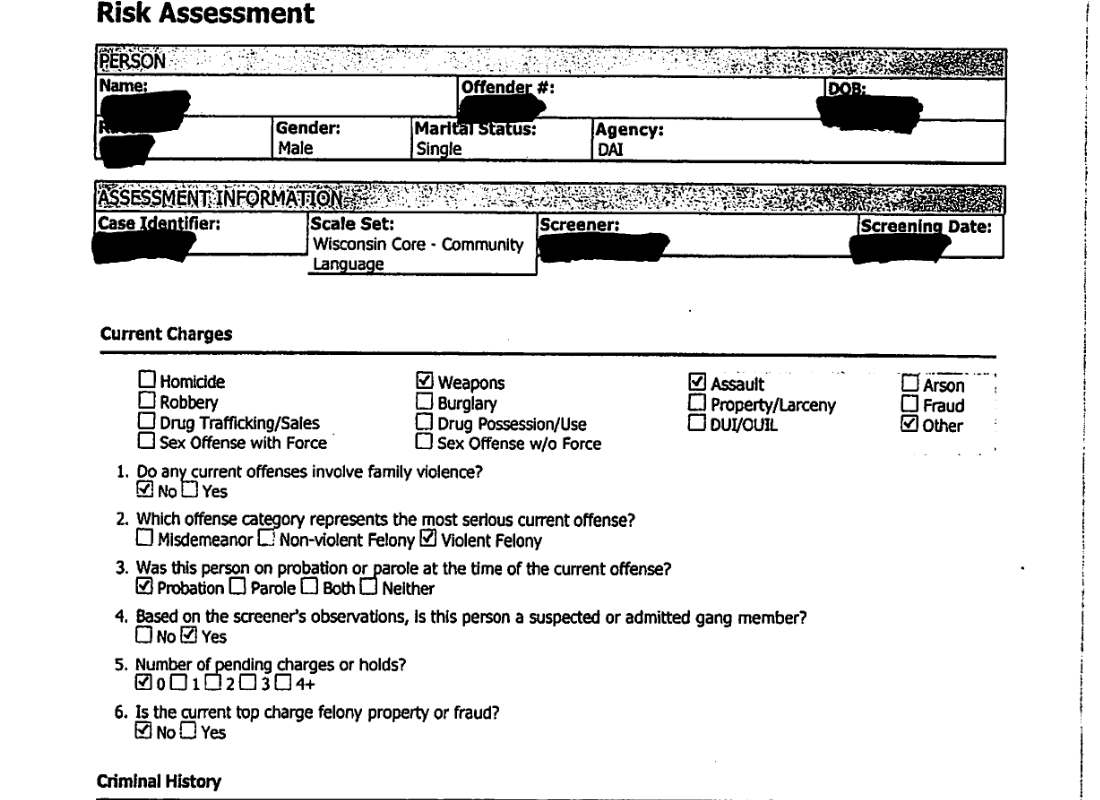
Correctional Offender Management Profiling for Alternative Sanctions (COMPAS)

Risk assessment software for rating a defendant’s risk of future crime (recidivism)
- Based on 137 features (Questionnaire)
  - Does not include race!
Commercial software developed by Northpointe, not publicly disclosed
Can be used for targeting treatment programs, bail determinations (judges), and in the course of sentencing decisions

→ Test of accuracy and racial bias by ProPublica (Angwin et al. 2016)

5 The COMPAS Case II

Source: https://www.documentcloud.org/documents/2702103-Sample-Risk-Assessment-COMPAS-CORE.html

6 The COMPAS Case III

Source: Corbett-Davies et al. (2017), Fig. 1, Distribution of risk scores for Broward County¹

7 The COMPAS Case IV

COMPAS Fairness Metrics (Rodolfa, Saleiro, and Ghani 2020)
Metric	Caucasian	African American
False Positive Rate (FPR)	23%	45%
False Negative Rate (FNR)	48%	28%
False Discovery Rate (FDR)	41%	37%

ProPublica focused on FPR and FNR
Northpointe’s response² put forward FDR
Is the model “simultaneously fair and unfair”?

8 The COMPAS Case V: Error rates

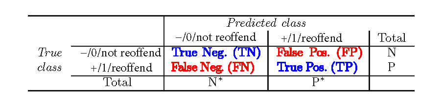
Source: modified from James et al. (2013), Ch. 4.4.3, Table 4.6, p. 148

\[ \text{FPR} = \frac{\text{False Positives (FP)}}{\text{False Positives (FP)} + \text{True Negatives (TN)}} \]

\[ \text{FNR} = \frac{\text{False Negatives (FN)}}{\text{False Negatives (FN)} + \text{True Positives (TP)}} \]

\[ \text{FDR} = \frac{\text{False Positives (FP)}}{\text{False Positives (FP)} + \text{True Positives (TP)}} \]

Intepreting the rates³

Exercise: Calculate the FPR, FNR, FDR!⁴

	0/not reoffend	1/reoffend
0/not reoffend	49 (TN)	41 (FP)	90 (N)
1/reoffend	7 (FN)	18 (TP)	25 (P)
	56 (N*)	59 (P*)	125 (total)

9 Examples of discrimination & bias: Exercise

What other examples of algorithms that discriminate have you heard of?

A few examples..

10 Fairness and Automated Decision-Making

ML increasingly used for guiding high-stakes decisions
Hopes
- Automated decision-making increases effectiveness and consistency?
- Protect against human subjectivity/deficiencies (Q: Examples?)
BUT various forms of (data) biases can be fed into the system
- Models trained on biased data learn to reproduce biases!

“In the context of decision-making, fairness is the absence of any prejudice or favoritism toward an individual or a group based on their inherent or acquired characteristics.” (Mehrabi et al. 2021)

11 Discrimination & protected attributes

11.1 Legal discrimination definitions (Barocas and Selbst 2016)

Disparate Treatment
- Intentionally treating an individual differently based on his/her membership in a protected class
Disparate Impact
- Negatively affecting members of a protected class more than others even if by a seemingly neutral policy
Q: Can you think of any attributes that are protected?

11.2 Explainable Discrimination

Discrimination: “a source for unfairness that is due to human prejudice and stereotyping based on the sensitive attributes, which may happen intentionally or unintentionally” (Mehrabi et al. 2021, 115:10)
- “while bias can be considered as a source for unfairness that is due to the data collection, sampling, and measurement” (Mehrabi et al. 2021, 115:10)
Explainable Discrimination: Differences in treatment and outcomes among different groups can be explained via some attributes and (sometimes) justified and are not considered illegal as a consequence
- UCI Adult dataset (Kamiran and Žliobaitė 2013): Dataset used in fairness domain where males on average have a higher annual income than females⁵
Q: What do you think is reverse discrimination?⁶
Q: Can you give other examples of explainable discrimination?⁷

11.3 Unexplainable Discrimination & Sources

Unexplainable Discrimination: Unexplainable discrimination in which the discrimination toward a group is unjustified and therefore considered illegal
- Direct discrimination: happens when protected attributes of individuals explicitly result in non-favorable outcomes toward them (e.g., race, sex, etc.)
  - see Table 3 (Mehrabi et al. 2021, 115:15)
- Indirect discrimination: individuals appear to be treated based on seemingly neutral and non-protected attributes; however, protected groups, or individuals, still get to be treated unjustly as a result of implicit effects from their protected attributes (e.g., residential zip code: Q:why?)
  - Q: Can you think of other examples of indirect discrimination?
Sources of discrimination
- Systemic discrimination: refers to policies/customs/behaviors that are a part of the culture or structure of an organization that may perpetuate discrimination against certain subgroups
- Statistical discrimination: a phenomenon where decision-makers use average group statistics to judge an individual belonging to that group

11.4 Protected attributes (U.S.)

Table 1 shows protected attributes in the US as defined by the Fair Housing Act (FHA) and Equal Credit Opportunity Act (ECOA)

Table 1: Protected attributes

Attribute	FHA	ECOA
Race	✓	✓
Color	✓	✓
National origin	✓	✓
Religion	✓	✓
Sex	✓	✓
Familial status	✓
Disability	✓
Exercised rights under CCPA		✓
Marital status		✓
Recipient of public assistance		✓
Age		✓

11.5 Protected attributes (Germany/Europe)

Allgemeines Gleichbehandlungsgesetz (AGG)⁸
Datenschutz-Grundverordnung (DSGVO)⁹
- “Die Verarbeitung personenbezogener Daten, aus denen die rassische und ethnische Herkunft, politische Meinungen, religiöse oder weltanschauliche Überzeugungen oder die Gewerkschaftszugehörigkeit hervorgehen, sowie die Verarbeitung von genetischen Daten, biometrischen** Daten zur eindeutigen Identifizierung einer natürlichen Person, Gesundheitsdaten oder Daten zum Sexualleben oder der sexuellen Orientierung einer natürlichen Person ist untersagt.” (DSGVO, Art. 9)
EU-directives against discrimination (z.B. 2000/43/EG, 2000/78/EG)
EU Artificial intelligence act

12 Biases

Source: Mehrabi et al. (2021, sec. 3.1)
Mehrabi et al. (2021) discuss a wide variety of biases (sometimes those biases are a bit hard to distinguish)
Often biases lie at the origin of discrimination and unfairness

12.1 Biases in a feed-back loop

Figure 1 visualizes the loop capturing the feedback between biases in data, algorithms, and user interaction.

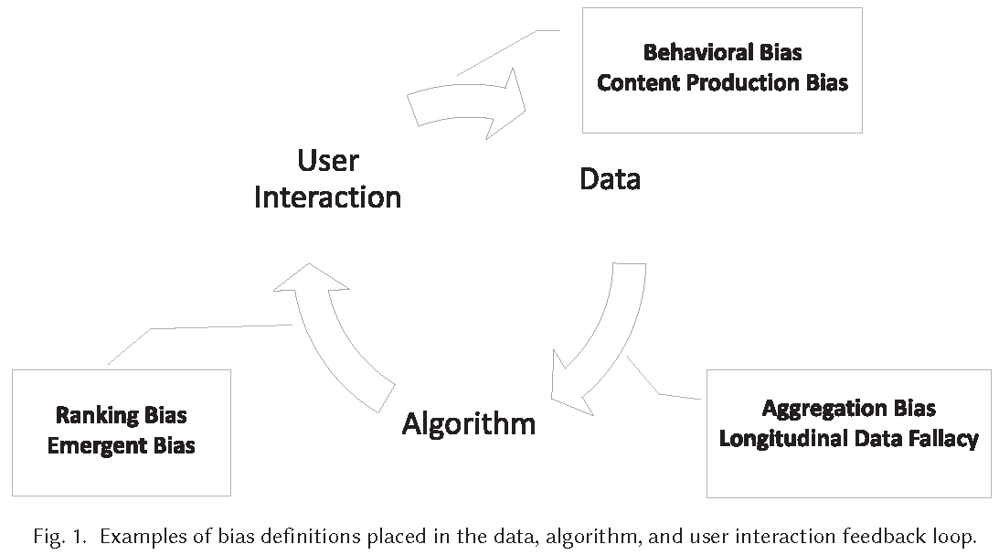
Figure 1: Source: Mehrabi et al. (2021), 115:4

Biases in data feed into algorithms that affect user interaction that feeds into data
Example of web search engine (Mehrabi et al. 2021, 115:4)
- Algorithm: Puts specific results at the top of its list and users tend to interact most with the top results
- User interaction: Interactions of users with items will then be collected by web search engine, and data will be used to make future decisions on how information should be presented based on popularity and user interest
- Data: Results at the top will become more and more popular, not because of the nature of the result but due to the biased interaction and placement of results by these algorithms
Q: Can you think of other examples?

12.2 Exercise: Biases in a feed-back loop

Q: Discuss with your neighbor on how/wether this feedback loop in Figure 2 exists in the case of the recidivism example.

Figure 2: Source: Mehrabi et al. (2021), 115:4

12.3 Biases: Data to Algorithm

Idea: Biases in the data affect our algorithm/model and its predictions
Measurement Bias: arises from how we choose, utilize, and measure particular features¹⁰
Omitted Variable/Feature Bias: occurs when one or more important variables [predictors] are left out of the model¹¹
Representation Bias: arises from how we sample from a population during data collection process¹²
Aggregation Bias (or ecological fallacy): arises when false conclusions are drawn about individuals from observing the entire population¹³
Sampling Bias (\(\approx\) representation bias): arises due to non-random sampling of units (in subgroups like race)
Longitudinal Data Fallacy: occurs when incorrect conclusions are drawn from time-dependent data¹⁴
Linking Bias: occurs when network-derived attributes misrepresent users’ true behavior¹⁵

Q: Can you think of concrete examples of how data biases may feed into algorithms?

12.4 Biases: Algorithm to User

Idea: Biases in the algorithm/model may affect users
Algorithmic Bias: bias is not present in the input data but purely produced by the algorithm, i.e., originates from design/modelling choices¹⁶
User Interaction Bias: type of bias that can not only be observant on the Web but also get triggered from two sources - the user interface and through the user itself by imposing his/her self-selected biased behavior and interaction¹⁷
Popularity Bias: Items that are more popular tend to be exposed/seen more but popularity can be gamed, e.g., fake reviews by humans/bots
Emergent Bias: results from shift in population, cultural values, or societal knowledge (Q: Example?)¹⁸
Evaluation Bias: due to faulty/inappropiate model evaluation¹⁹

Q: Can you think of other concrete examples of algorithm biases?

12.5 Biases: User to Data

Idea: Biases occuring when data is collected on users
Historical Bias: Existing bias (e.g., inequality between groups) can seep into ML model from data generation process (even given a perfect sampling and feature selection)²⁰
Population Bias: arises when data is collected on a different population (e.g., Facebook users) than target population (e.g., Twitter users)²¹
Self-selection Bias: a subtype of selection or sampling bias in which subjects of the research select themselves²²
Social Bias: happens when others’ actions affect our judgment²³
Behavioral Bias: arises from different user behavior across platforms, contexts, or different datasets²⁴
Temporal Bias: arises from differences in populations over time²⁵
Content Production Bias: arises from structural, lexical, semantic, and syntactic differences in the contents generated by users²⁶

12.6 Exercise: Biases

Breakout rooms/Group discussion: Mehrabi et al. (2021) discuss an overwhelming, sometimes confusing amount of biases. Please go through the previous three slides on Data to Algoritm, Algorithm to User and User to Data biases (cf. Section 12.3, Section 12.4 and Section 12.5)
1. Discuss and explain these biases to each other in the group.
2. What biases are the ones that are commonly discussed?
3. What biases are especially relevant thinking of the outcome \(Y\) you want to predict with your model? (if you don’t have a ML project discuss the Compas example)

Solution(s)

Sampling bias, measurement bias, omitted variable/feature bias
Potentially, we are most concerned with User to Data and Data to Algoritm. For instance, sampling bias is usually a concern with any machine learning model we built for humans.

13 Algorithmic fairness definitions

13.1 Fairness definitions (1)

No universal definition of fairness (Saxena 2019)
Fairness: “absence of any prejudice or favoritism towards an individual or a group based on their intrinsic or acquired traits in the context of decision-making” (Saxena et al. 2019)
Many different definitions of fairness (Mehrabi et al. 2021; Verma and Rubin 2018)

13.2 Fairness definitions (2): Equality of Treatment

Fairness through Unawareness²⁷
- “An algorithm is fair as long as any protected attributes A are not explicitly used in the decision-making process” (Grgic-Hlaca et al. 2016; Kusner et al. 2017)
  - Blindness is ineffective (Dwork et al. 2012): Redundant encoding²⁸, reduced utility²⁹
vs. Fairness through Awareness³⁰
- “An algorithm is fair if it gives similar predictions to similar individuals” (Dwork et al. 2012; Kusner et al. 2017), i.e., two individuals who are similar with respect to a similarity (inverse distance) metric defined for a particular task should receive a similar outcome.

13.3 Fairness definitions (2): Equality of Outcomes

Demographic/Statistical Parity³¹ [Dwork et al. (2012); Kusner et al. (2017)]: people in both protected and unprotected groups should have equal probability of being assigned to a positive outcome (Verma and Rubin 2018)³²
- Can be exploited by biased adversaries (Dwork et al. 2012): only ensures that acceptance rates are equal** across groups – but says nothing about who is being accepted (creates loopholes that can be manipulated)
  - Reverse tokenism & Self-fulfilling prophecy³³
Conditional Statistical Parity
- Demographic parity holds given a set of legitimate factors³⁴
See discussions in Mehrabi et al. (2021) (Section 4) and Verma and Rubin (2018) for more definitions…

13.4 Fairness definitions (4): overview

Fairness definitions fall into different types as shown in Table in Figure 3.

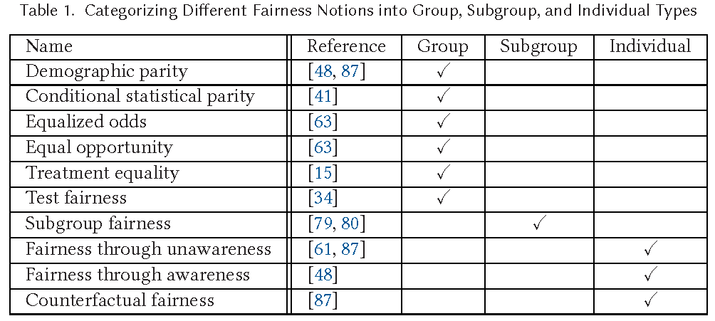
Figure 3: Source: Mehrabi et al. (2021), 115:4

(1) Individual Fairness: Give similar predictions to similar individuals
(2) Group Fairness: Treat different groups equally
(3) Subgroup Fairness: pick a group fairness constraint like equalizing false positives and asks whether this constraint holds over a large collection of subgroups

13.5 Fairness definitions (5): Equality of Errors

Given a model, evaluation data and groups defined by protected attributes, how can we “define” fairness (more adequately)?

13.6 Fairness definitions (6): Sufficiency

Given groups \(g\) defined by protected attributes…

Predictive Parity
- Equalize \(FDR_g = \frac{FP_g}{FP_g + TP_g}\)³⁵
\(FOR_g\)³⁶
- Equalize \(FOR_g = \frac{FN_g}{FN_g + TN_g}\)
Sufficiency³⁷
- Equalize \(FDR_g\) and \(FOR_g\)

\(\rightarrow\) \(\sim\)Perspective of decision-maker³⁸

		Predicted	class
		0	1
True	0	TN	FP	N’
class	1	FN	TP	P’
		N	P

13.7 Fairness definitions (7): Equalized Odds

Given groups \(g\) defined by protected attributes…

Predictive Equality³⁹
- Equalize \(FPR_g = \frac{FP_g}{FP_g + TN_g}\) or \(TNR\)
Equal Opportunity⁴⁰
- Equalize \(FNR_g = \frac{FN_g}{FN_g + TP_g}\) or \(TPR\)⁴¹
Equalized Odds⁴²
- Equalize \(FNR_g\) (or \(TPR\)) and \(FPR_g\) (or \(TNR\))

\(\rightarrow\) \(\sim\)Perspective of affected individual⁴³

		Predicted	class
		0	1
True	0	TN	FP	N’
class	1	FN	TP	P’
		N	P

13.8 Fairness definitions (8): Accuracy Equality

Given groups \(g\) defined by protected attributes…

Overall Accuracy Equality⁴⁴
- Equalize accuracy: \(\frac{TP_g+TN_g}{TP_g+FP_g+TN_g+FN_g}\)
Treatment Equality⁴⁵
- Equalize \(\frac{FP_g}{FN_g}\)⁴⁶

		Predicted	class
		0	1
True	0	TN	FP	N’
class	1	FN	TP	P’
		N	P

13.9 Fairness definitions (9): Group disparity measures

Group disparity measures (Saleiro et al. 2018)⁴⁷
Examples:
- \(FDR \, disp = \frac{FDR_{group}}{FDR_{basegroup}}\)⁴⁸
- \(FPR \, disp = \frac{FPR_{group}}{FPR_{basegroup}}\)⁴⁹

Range of disparity values that can be considered fair⁵⁰

\[ \tau \leq Disparity \, Measure \leq \frac{1}{\tau} \]

13.10 Fairness Trade-offs: Impossibility of Fairness

“When the base rates differ by protected group and when there is not separation, one cannot have both conditional use accuracy equality⁵¹ and equality in the false negative and false positive rates” (Berk et al. 2021, 20)⁵²
- Equality of \(FDR\), \(FOR\) and \(FNR\), \(FPR\) across groups hardly possible in practice
- Trade-off between Sufficiency and Equalized Odds

14 Tidymodels

14.1 Tidymodels: Accuracy equality (1)

Key Functions
- metrics_combined <- metric_set(...): Define and save metric set that includes relevant metrics
- Metrics
  - accuracy(): Proportion of correctly predicted cases
    - \((TN + TP)/(TN + TP + FN + FP)\)
  - precision() or ppv(): Proportion positive correctly identified (= \(TP\)) among all positive predictions (\(P*\))
    - \(TP/P*= \text{Positive predictive value}\)
  - recall() or sens(): Proportion positive correctly identified (= \(TP\)) among all actual positives (\(P\))
    - \(TP/P = \text{True positive rate}\)
  - f_meas(): Harmonic mean of precision and recall⁵³
  - spec() or npv(): Proportion negative correctly identified (= \(TN\)) among all negative predictions (\(N*\))
    - \(TN/N*= \text{Specificity/Negative predictive value}\)
    - 1 - spec(): Proportion positive NOT correctly identified (= \(FP\)) among all actual negatives (\(N\))
      - \(FP/N = \text{FPR} = \text{False positive rate}\)

Open confusion matrix

14.2 Tidymodels: Accuracy equality (2)

We can simply group_by the predictions and calculate the accuracy for data subsets (e.g., individuals of different race)

metrics_combined <- metric_set(accuracy, recall, precision, f_meas, spec)

data_test %>%
      augment(x = fit_lr, type.predict = "response") %>%
      group_by(race) %>%
      metrics_combined(truth = reoffend_factor, estimate = .pred_class)

14.3 Tidymodels: Fairness (1)

Fairness functions in tidymodels (values of 0 indicate parity across groups)
- Have to be added to metric_set() including group variable, e.g., race
- equal_opportunity()⁵⁴
- equalized_odds()⁵⁵
- demographic_parity()⁵⁶
- You can also create groupwise metrics yourself..

metrics_combined <- metric_set(
    equal_opportunity(race),
    equalized_odds(race),
    demographic_parity(race))

data_test %>%
    augment(x = fit_lr, type.predict = "response") %>%
    metrics_combined(truth = reoffend_factor, estimate = .pred_class)

15 Lab: Assessing fairness in R

See here for a description of the data and illustration of how to explore the data. Below we explore how to assess algorithmic fairness for the variable race.

Overview of Compas dataset variables

id: ID of prisoner, numeric
name: Name of prisoner, factor
compas_screening_date: Date of compass screening, date
decile_score: the decile of the COMPAS score, numeric
reoffend: whether somone reoffended/recidivated (=1) or not (=0), numeric
reoffend_factor: same but factor variable
age: a continuous variable containing the age (in years) of the person, numeric
age_cat: age categorized
priors_count: number of prior crimes committed, numeric
sex: gender with levels “Female” and “Male”, factor
race: race of the person, factor
juv_fel_count: number of juvenile felonies, numeric
juv_misd_count: number of juvenile misdemeanors, numeric
juv_other_count: number of prior juvenile convictions that are not considered either felonies or misdemeanors, numeric

We first import the data into R:

# install.packages(pacman)
pacman::p_load(tidyverse,
               tidymodels,
               knitr,
               kableExtra,
               DataExplorer,
               visdat,
               naniar)

rm(list=ls())
load(url(sprintf("https://docs.google.com/uc?id=%s&export=download",
                         "1gryEUVDd2qp9Gbgq8G0PDutK_YKKWWIk")))

Explore and visualize the race variable.

Q: What do we find?

table(data$race, useNA = "always") %>%
  kable(col.names = c("Race", "Frequency"))

Race	Frequency
African-American	3696
Asian	32
Caucasian	2454
Hispanic	637
Native American	18
Other	377
NA	0

data %>%
  ggplot(aes(x = fct_infreq(race))) + # fct_infreq(): reoder according to frequency
    geom_bar() + # create barplot
    geom_text(stat = "count", # add proportions
            aes(label = round((after_stat(count)) / sum(after_stat(count)), 2), 
                vjust = -0.5))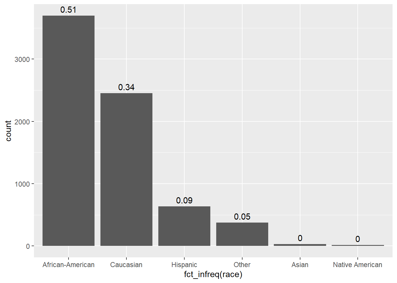

15.1 Estimate model

Below we estimate the MLM that we want to evaluate later on (using a workflow and without resampling).

# Extract data with missing outcome
  data_missing_outcome <- data %>% filter(is.na(reoffend_factor))
  dim(data_missing_outcome)

[1] 614  14

# Omit individuals with missing outcome from data
  data <- data %>% drop_na(reoffend_factor) # ?drop_na
  dim(data)

[1] 6600   14

# Split the data into training and test data
  data_split <- initial_split(data, prop = 0.80)
  data_split # Inspect

<Training/Testing/Total>
<5280/1320/6600>

# Extract the two datasets
  data_train <- training(data_split)
  data_test <- testing(data_split) # Do not touch until the end!

  
# Define a recipe for preprocessing (taken from above)
  recipe_lr <- recipe(reoffend_factor ~ age + priors_count + race, data = data_train) %>%
    recipes::update_role(race, new_role = "id") # keep but don't use in model
  
# Define a model
  model_lr <- logistic_reg() %>% # logistic model
            set_engine("glm") %>% # define lm package/function
            set_mode("classification")
  
  
# Define a workflow
  workflow1 <- workflow() %>% # create empty workflow
    add_recipe(recipe_lr) %>% # add recipe
    add_model(model_lr) # add model  
  
# Fit the workflow (including recipe and model)
  fit_lr <- workflow1 %>% fit(data = data_train)


# Add prediction to training data and test data 
  data_train <- data_train %>% augment(x = fit_lr, type.predict = "response")
  data_test <- data_test %>% augment(x = fit_lr, type.predict = "response")

Subsequently, we can use the obtained datasets that include the predictions to explore algorithmic bias.

15.1.1 Accuracy across groups

Below we start by estimating different accuracy measures across groups. We compute them for the full test data as benchmark and subsequently for the different groups using race and sex (male, female) as grouping variables. We filter out everyone who is not African American or Caucasian (filter(race=="African-American"|race=="Caucasian")). We already added the predictions to the data_test above.

# Confusion matrix
  data_test %>%
      conf_mat(truth = reoffend_factor, 
               estimate = .pred_class) %>% 
  pluck("table") %>% t() %>% addmargins()

     Prediction
Truth   no  yes  Sum
  no   498  196  694
  yes  222  404  626
  Sum  720  600 1320

# Accuracy measures across groups
  metrics_combined <- metric_set(accuracy, recall, precision, f_meas, yardstick::spec) # Use several metrics
  
# Metrics for teh full testset (as benchmark)
  data_test %>%
    metrics_combined(truth = reoffend_factor, estimate = .pred_class)

# A tibble: 5 × 3
  .metric   .estimator .estimate
  <chr>     <chr>          <dbl>
1 accuracy  binary         0.683
2 recall    binary         0.718
3 precision binary         0.692
4 f_meas    binary         0.704
5 spec      binary         0.645

And now for the groups!⁵⁷

# Across groups: Race
data_test %>%
  filter(race=="African-American"|race=="Caucasian") %>%
      group_by(race) %>%
      metrics_combined(truth = reoffend_factor, estimate = .pred_class) %>%
  pivot_wider(names_from = race, values_from = .estimate)

# A tibble: 5 × 4
  .metric   .estimator `African-American` Caucasian
  <chr>     <chr>                   <dbl>     <dbl>
1 accuracy  binary                  0.688     0.670
2 recall    binary                  0.625     0.792
3 precision binary                  0.677     0.688
4 f_meas    binary                  0.65      0.736
5 spec      binary                  0.742     0.503

# Across groups: Race
data_test %>%
      group_by(sex) %>%
      metrics_combined(truth = reoffend_factor, estimate = .pred_class)%>%
  pivot_wider(names_from = sex, values_from = .estimate)

# A tibble: 5 × 4
  .metric   .estimator Female  Male
  <chr>     <chr>       <dbl> <dbl>
1 accuracy  binary      0.688 0.682
2 recall    binary      0.761 0.705
3 precision binary      0.738 0.678
4 f_meas    binary      0.749 0.691
5 spec      binary      0.574 0.659

Visualizing often facilitates interpretation a shown in Figure 4. What can we see in Figure 4?

# Visualize
  p1 <- data_test %>%
    metrics_combined(truth = reoffend_factor, estimate = .pred_class) %>%
    ggplot(aes(x = .metric, y = .estimate, color = .metric)) +
    geom_point(size = 3) +
    theme_minimal() + 
  theme(axis.text.x = element_text(angle = 45, hjust = 1)) +
  scale_y_continuous(breaks = seq(0, 1, by = 0.1),
                     limits = c(0,1))
  
  
  p2 <- data_test %>%
    filter(race=="African-American"|race=="Caucasian") %>%
      group_by(race) %>%
      metrics_combined(truth = reoffend_factor, estimate = .pred_class) %>%
    ungroup() %>%
    ggplot(aes(x = .metric, y = .estimate, color = race, group = race)) +
    geom_point(size = 3, position = position_dodge(width = 0.3)) +
    geom_line(position = position_dodge(width = 0.3))+
    theme_minimal() + 
    theme(axis.text.x = element_text(angle = 45, hjust = 1)) +
  scale_y_continuous(breaks = seq(0, 1, by = 0.1),
                     limits = c(0,1))
  
  
 # Across groups: sex
  p3 <- data_test %>%
      group_by(sex) %>%
      metrics_combined(truth = reoffend_factor, estimate = .pred_class) %>%
    ungroup() %>%
    ggplot(aes(x = .metric, y = .estimate, color = sex, group = sex)) +
    geom_point(size = 3, position = position_dodge(width = 0.3)) +
    geom_line(position = position_dodge(width = 0.3))+
    theme_minimal() + theme(axis.text.x = element_text(angle = 45, hjust = 1))+
  scale_y_continuous(breaks = seq(0, 1, by = 0.1),
                     limits = c(0,1)) 
  
library(patchwork)
  
 p1 + p2+ p3+
  plot_layout(axis_titles = "collect",
              design = "AAAAAA 
  BBBCCC")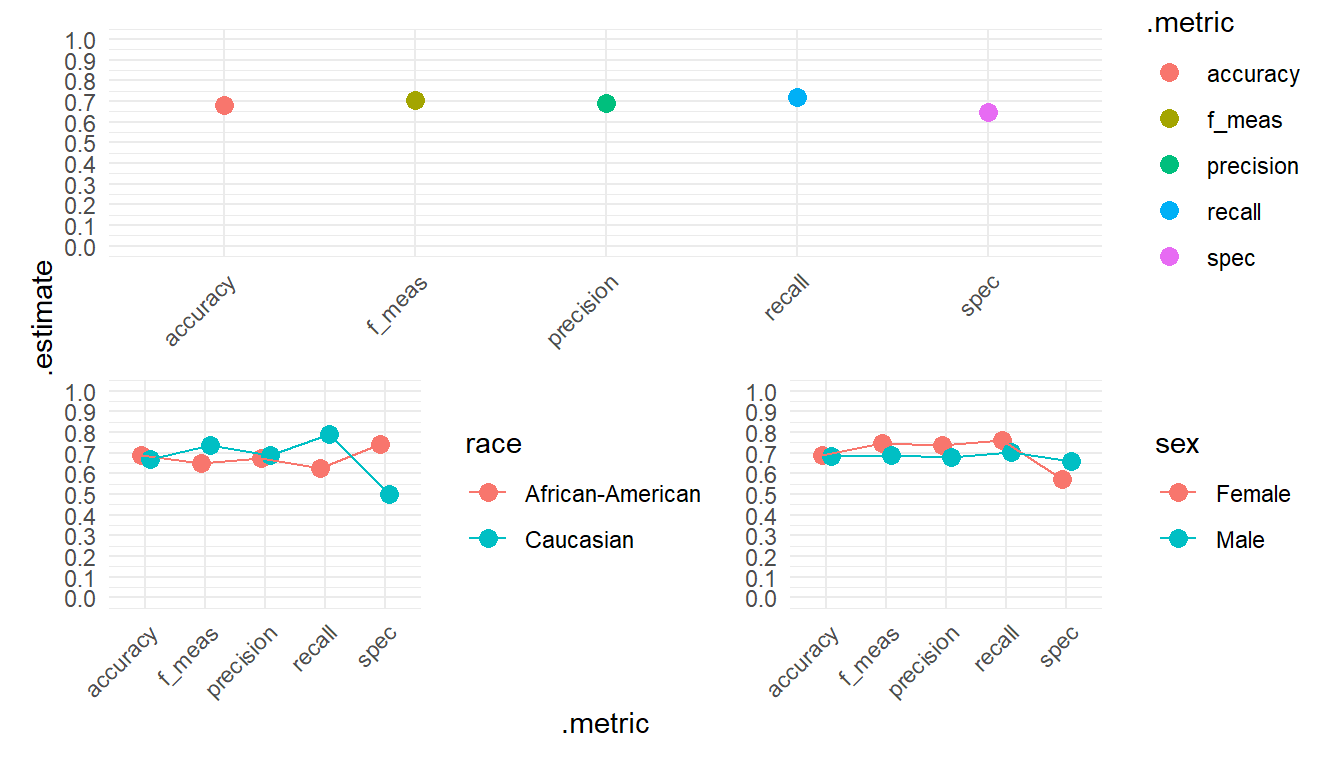

Figure 4: Visualizing accuracy overall and across groups (race, sex)

15.1.2 Fairness across groups

In addition, we can calculate different fairness metrics and visualize them in Figure 5. Q: What can we see in the graphs?⁵⁸

Equal opportunity is satisfied when a model’s predictions have the same true positive and false negative rates across protected groups. A value of 0 indicates parity across groups.
Equalized odds is satisfied when a model’s predictions have the same false positive, true positive, false negative, and true negative rates across protected groups. A value of 0 indicates parity across groups.
Demographic parity is satisfied when a model’s predictions have the same predicted positive rate across groups. A value of 0 indicates parity across groups.

# Specify metrics
  # Certain metrics are calculated for specific grouping variables
  # e.g., equal_opportunity(age_cat)
  metrics_combined <- metric_set(
                                      equal_opportunity(race),
                                      equalized_odds(race),
                                      demographic_parity(race),
                                      equal_opportunity(sex),
                                      equalized_odds(sex),
                                      demographic_parity(sex)) # Use several metrics



# Test data: Metrics
  data_test %>%
    filter(race=="African-American"|race=="Caucasian") %>%
    metrics_combined(truth = reoffend_factor, estimate = .pred_class) %>%
    ggplot(aes(x = .metric, y = .estimate, color = .by, group = .by)) +
    geom_point(size = 3, position = position_dodge(width = 0.3)) +
    geom_line(position = position_dodge(width = 0.3))+
    theme_minimal() +
  scale_y_continuous(breaks = seq(0, 1, by = 0.1),
                     limits = c(0,1))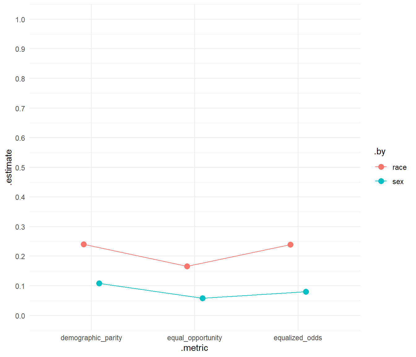

Figure 5: Visualizing fairness across groups (race, sex)

15.1.3 More metrics (fairness)

Below, we calculate more rates, for now ignoring groups!

# Define accuracy metrics
  metrics_combined <- metric_set(accuracy, recall, precision, f_meas, spec) # Use several metrics
  
# Metrics for full testset (as benchmark)
  data_test %>%
    metrics_combined(truth = reoffend_factor, estimate = .pred_class) %>%
    add_row(.metric = "FPR (1 - specificity)", 
            .estimator="binary", .estimate = 1-.$.estimate[5]) %>%
    add_row(.metric = "FNR (1 − recall/TPR)", 
            .estimator="binary", .estimate = 1-.$.estimate[2]) %>%
    add_row(.metric = "TNR (1 - FPR)", 
            .estimator="binary", .estimate = 1-.$.estimate[6]) %>%
    mutate(.metric = recode(.metric,
                            "recall" = "recall/TPR"))

# A tibble: 8 × 3
  .metric               .estimator .estimate
  <chr>                 <chr>          <dbl>
1 accuracy              binary         0.683
2 recall/TPR            binary         0.718
3 precision             binary         0.692
4 f_meas                binary         0.704
5 spec                  binary         0.645
6 FPR (1 - specificity) binary         0.355
7 FNR (1 − recall/TPR)  binary         0.282
8 TNR (1 - FPR)         binary         0.645

Then we calculate these rates grouping the data according to race. Unfortunately, the code above does not work with group_by(), hence, we do it for subsets of data and merge them later on. Importantly, these are the metric based on our predictive logistic regression model.

# Accuracy measures across groups
  metrics_combined <- metric_set(accuracy, recall, precision, f_meas, spec)
  
# Metrics for thh full testset (as benchmark)
metrics_African_American <- 
    data_test %>%
    filter(race=="African-American") %>%
    metrics_combined(truth = reoffend_factor, estimate = .pred_class) %>%
    add_row(.metric = "FPR (1 - specificity)", 
            .estimator="binary", .estimate = 1-.$.estimate[5]) %>%
    add_row(.metric = "FNR (1 − recall/TPR)", 
            .estimator="binary", .estimate = 1-.$.estimate[2]) %>%
    add_row(.metric = "TNR (1 - FPR)", 
            .estimator="binary", .estimate = 1-.$.estimate[6]) %>%
    mutate(.metric = recode(.metric,
                            "recall" = "recall/TPR")) %>%
  rename("African_American" = ".estimate")

metrics_Caucasian <- 
    data_test %>%
    filter(race=="Caucasian") %>%
    metrics_combined(truth = reoffend_factor, estimate = .pred_class) %>%
    add_row(.metric = "FPR (1 - specificity)", 
            .estimator="binary", .estimate = 1-.$.estimate[5]) %>%
    add_row(.metric = "FNR (1 − recall/TPR)", 
            .estimator="binary", .estimate = 1-.$.estimate[2]) %>%
    add_row(.metric = "TNR (1 - FPR)", 
            .estimator="binary", .estimate = 1-.$.estimate[6]) %>%
    mutate(.metric = recode(.metric,
                            "recall" = "recall/TPR")) %>%
  rename("Caucasian" = ".estimate")

metrics_all <- 
  bind_cols(metrics_African_American %>% select(-.estimator),
            metrics_Caucasian %>% select(-.estimator, -.metric))

metrics_all

# A tibble: 8 × 3
  .metric               African_American Caucasian
  <chr>                            <dbl>     <dbl>
1 accuracy                         0.688     0.670
2 recall/TPR                       0.625     0.792
3 precision                        0.677     0.688
4 f_meas                           0.65      0.736
5 spec                             0.742     0.503
6 FPR (1 - specificity)            0.258     0.497
7 FNR (1 − recall/TPR)             0.375     0.208
8 TNR (1 - FPR)                    0.742     0.503

16 Exercise/Homework: Fairness

Above we discovered that ethnic groups (African-Americans vs. Caucasians) are treated (slightly) differently by our own model. Please first take the time to read and understand the lab in Section 15.
Then, please explore whether you can find similar patterns (unfairness) for other socio-demographic variables, namely age_cat using our prediction model. You can use the code from our lab Section 15 and adapt it accordingly, e.g., change the grouping variable.

table(data$race)


African-American            Asian        Caucasian         Hispanic 
            3380               29             2235              588 
 Native American            Other 
              16              352

table(data$sex)


Female   Male 
  1293   5307

table(data$age_cat)


        25 - 45 Greater than 45    Less than 25 
           3743            1466            1391

Solution

# install.packages(pacman)
pacman::p_load(tidyverse,
               tidymodels,
               knitr,
               kableExtra,
               DataExplorer,
               naniar)

rm(list=ls())
load(url(sprintf("https://docs.google.com/uc?id=%s&export=download",
                 "1gryEUVDd2qp9Gbgq8G0PDutK_YKKWWIk")))


# Extract data with missing outcome
data_missing_outcome <- data %>% filter(is.na(reoffend_factor))
dim(data_missing_outcome)

# Omit individuals with missing outcome from data
data <- data %>% drop_na(reoffend_factor) # ?drop_na
dim(data)

# Split the data into training and test data
data_split <- initial_split(data, prop = 0.80)
data_split # Inspect


# Extract the two datasets
data_train <- training(data_split)
data_test <- testing(data_split) # Do not touch until the end!


# Define a recipe for preprocessing (taken from above)
recipe_lr <- recipe(reoffend_factor ~ priors_count + age, data = data_train)

# Define a model
model_lr <- logistic_reg() %>% # logistic model
  set_engine("glm") %>% # define lm package/function
  set_mode("classification")


# Define a workflow
workflow1 <- workflow() %>% # create empty workflow
  add_recipe(recipe_lr) %>% # add recipe
  add_model(model_lr) # add model  

# Fit the workflow (including recipe and model)
fit_lr <- workflow1 %>% fit(data = data_train)


# Add prediction to training data and test data 
data_train <- data_train %>% augment(x = fit_lr, type.predict = "response")
data_test <- data_test %>% augment(x = fit_lr, type.predict = "response")




# Accuracy measures across groups
metrics_combined <- metric_set(accuracy, recall, precision, f_meas, yardstick::spec) # Use several metrics

# Metrics for teh full testset (as benchmark)
data_test %>%
  metrics_combined(truth = reoffend_factor, estimate = .pred_class)




# Across groups: age_cat
data_test %>%
  group_by(age_cat) %>%
  metrics_combined(truth = reoffend_factor, estimate = .pred_class) %>%
  pivot_wider(names_from = age_cat, values_from = .estimate)




# Specify metrics
# Certain metrics are calculated for specific grouping variables
# e.g., equal_opportunity(age_cat)
metrics_combined <- metric_set(
  equal_opportunity(age_cat),
  equalized_odds(age_cat),
  demographic_parity(age_cat),
  equal_opportunity(sex),
  equalized_odds(sex),
  demographic_parity(sex)) # Use several metrics



# Test data: Metrics
data_test %>%
  metrics_combined(truth = reoffend_factor, estimate = .pred_class) %>%
  ggplot(aes(x = .metric, y = .estimate, color = .by, group = .by)) +
  geom_point(size = 3, position = position_dodge(width = 0.3)) +
  geom_line(position = position_dodge(width = 0.3))+
  theme_minimal() +
  scale_y_continuous(breaks = seq(0, 1, by = 0.1),
                     limits = c(0,1))

17 Lab: Northpointe Compas score fairness

Beware: We are not dealing with the original data by probublica but added a few missing on the outcome for teaching purposes. This may change estimates of different rates and fairness metrics.

Northpointe’s predictions are based on the Compas score that is stored in the variable decile_score. Below we visualize the distribution in Figure 6 both for all individuals and small multiples grouped according to race. We can see that the distribution differs strongly across groups of race.

library(ggplot2)
library(patchwork)
p1 <- ggplot(data = data, 
             aes(x = decile_score)) + 
  geom_histogram(binwidth = 1) +
  scale_x_continuous(breaks = 0:10) + 
  theme_light()
p2 <- ggplot(data = data, 
             aes(x = decile_score)) + 
  geom_histogram(binwidth = 1) +
  scale_x_continuous(breaks = 0:10) + 
  theme_light() +
  facet_wrap(~race)


p1+p2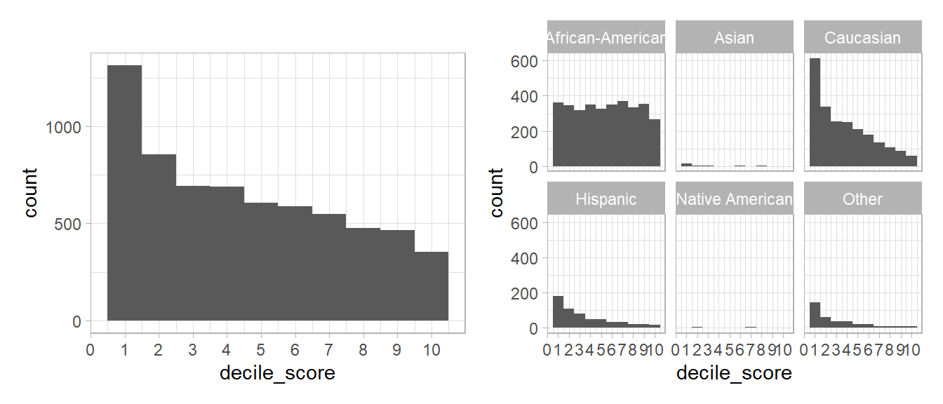

Figure 6: Distribution of reoffend (recidivism)

Then we use decile_score to obtain predictions for each individual where they predicted to reoffend if decile_score > 5 and predicted NOT to reoffend if decile_score <= 5. We simply do this for all the data. Since, the Compas score is provided for all individuals in the dataset and we are not training/testing a machine learning model, we can simply use all the data to evaluate accuracy.

data$.pred_class_compas <- factor(ifelse(data$decile_score > 5, "yes", "no"))
table(data$decile_score, data$.pred_class_compas)

    
       no  yes
  1  1315    0
  2   858    0
  3   694    0
  4   690    0
  5   607    0
  6     0  588
  7     0  550
  8     0  478
  9     0  467
  10    0  353

Now we can also calculate accuracy measures comparing the Compas prediction (.pred_class_compas based on decile_score) with the true outcome stored in reoffend_factor (cf. Section 15.1.1). Importantly, here we use all the data stored in data (not only data_test).

# Confusion matrix
  data %>%
      conf_mat(truth = reoffend_factor, 
               estimate = .pred_class_compas) %>% 
  pluck("table") %>% t() %>% addmargins()

     Prediction
Truth   no  yes  Sum
  no  2641  781 3422
  yes 1523 1655 3178
  Sum 4164 2436 6600

# Accuracy measures across groups
  metrics_combined <- metric_set(accuracy, recall, precision, f_meas, spec)
  
# Metrics for teh full testset (as benchmark)
  data %>%
    metrics_combined(truth = reoffend_factor, estimate = .pred_class_compas)

# A tibble: 5 × 3
  .metric   .estimator .estimate
  <chr>     <chr>          <dbl>
1 accuracy  binary         0.651
2 recall    binary         0.772
3 precision binary         0.634
4 f_meas    binary         0.696
5 spec      binary         0.521

# Across groups: Race
data %>%
  filter(race=="African-American"|race=="Caucasian") %>%
      group_by(race) %>%
      metrics_combined(truth = reoffend_factor, estimate = .pred_class_compas) %>%
  pivot_wider(names_from = race, values_from = .estimate)

# A tibble: 5 × 4
  .metric   .estimator `African-American` Caucasian
  <chr>     <chr>                   <dbl>     <dbl>
1 accuracy  binary                  0.638     0.666
2 recall    binary                  0.658     0.857
3 precision binary                  0.587     0.663
4 f_meas    binary                  0.621     0.748
5 spec      binary                  0.621     0.405

Subsequently, we also visualize those metrics as in Section 15.1.1. What can we see in Figure 4?

# Visualize
  p1 <- data %>%
    metrics_combined(truth = reoffend_factor, estimate = .pred_class_compas) %>%
    ggplot(aes(x = .metric, y = .estimate, color = .metric)) +
    geom_point(size = 3) +
    theme_minimal() + 
  theme(axis.text.x = element_text(angle = 45, hjust = 1)) +
  scale_y_continuous(breaks = seq(0, 1, by = 0.1),
                     limits = c(0,1))
  
  
  p2 <- data %>%
    filter(race=="African-American"|race=="Caucasian") %>%
      group_by(race) %>%
      metrics_combined(truth = reoffend_factor, estimate = .pred_class_compas) %>%
    ungroup() %>%
    ggplot(aes(x = .metric, y = .estimate, color = race, group = race)) +
    geom_point(size = 3, position = position_dodge(width = 0.3)) +
    geom_line(position = position_dodge(width = 0.3))+
    theme_minimal() + 
    theme(axis.text.x = element_text(angle = 45, hjust = 1)) +
  scale_y_continuous(breaks = seq(0, 1, by = 0.1),
                     limits = c(0,1))
  
  
 # Across groups: sex
  p3 <- data %>%
      group_by(sex) %>%
      metrics_combined(truth = reoffend_factor, estimate = .pred_class_compas) %>%
    ungroup() %>%
    ggplot(aes(x = .metric, y = .estimate, color = sex, group = sex)) +
    geom_point(size = 3, position = position_dodge(width = 0.3)) +
    geom_line(position = position_dodge(width = 0.3))+
    theme_minimal() + theme(axis.text.x = element_text(angle = 45, hjust = 1))+
  scale_y_continuous(breaks = seq(0, 1, by = 0.1),
                     limits = c(0,1)) 
  
library(patchwork)
  
 p1 + p2+ p3+
  plot_layout(axis_titles = "collect",
              design = "AAAAAA 
  BBBCCC")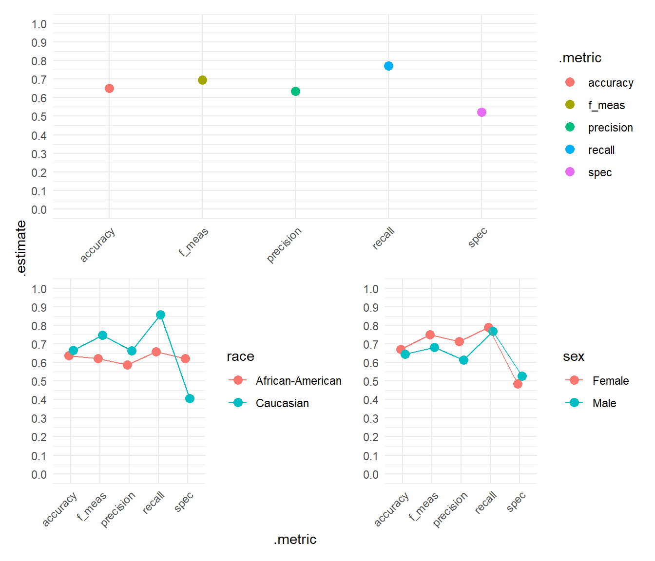

Figure 7: Compas prediction: Visualizing accuracy overall and across groups (race, sex)

And we also calculate the fairness metrics include in tidymodels for the Compas score (cf. Section 15.1.2). Figure 8 visualizes different fairness metrics but now based on the predictions using the Compas score. How do they compare to our own simple model Section 15.1.2?

# Specify metrics
  # Certain metrics are calculated for specific grouping variables
  # e.g., equal_opportunity(age_cat)
  metrics_combined <- metric_set(
                                      equal_opportunity(race),
                                      equalized_odds(race),
                                      demographic_parity(race),
                                      equal_opportunity(sex),
                                      equalized_odds(sex),
                                      demographic_parity(sex)) # Use several metrics



# Test data: Metrics
  data %>%
    filter(race=="African-American"|race=="Caucasian") %>%
    metrics_combined(truth = reoffend_factor, estimate = .pred_class_compas) %>%
    ggplot(aes(x = .metric, y = .estimate, color = .by, group = .by)) +
    geom_point(size = 3, position = position_dodge(width = 0.3)) +
    geom_line(position = position_dodge(width = 0.3))+
    theme_minimal() +
  scale_y_continuous(breaks = seq(0, 1, by = 0.1),
                     limits = c(0,1))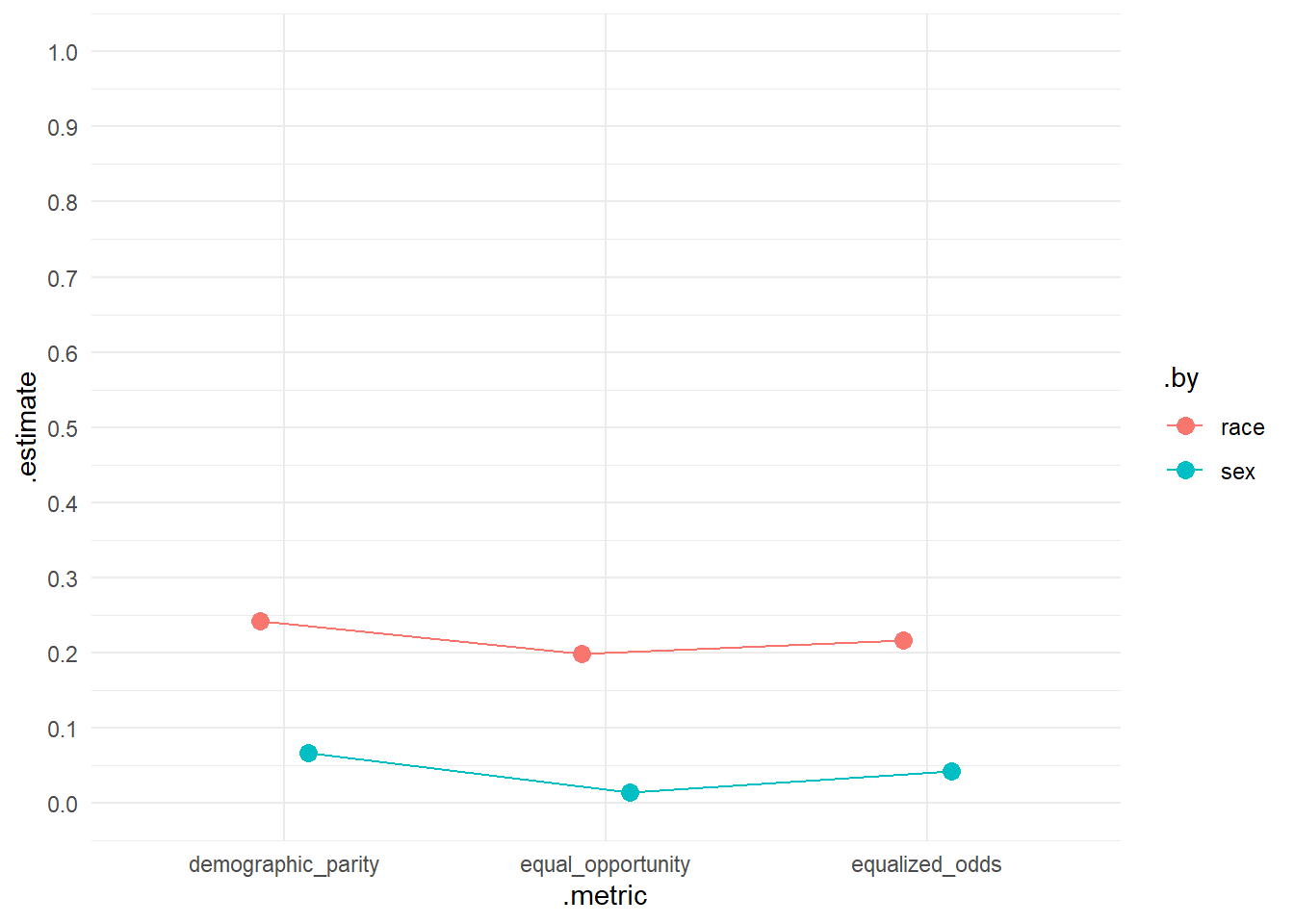

Figure 8: Compas prediction: Visualizing fairness across groups (race, sex)

Finally, we can calculate more metrics both for African-Americans and Caucasions (cf. Section 15.1.3).

# Accuracy measures across groups
  metrics_combined <- metric_set(accuracy, recall, precision, f_meas, spec)
  
# Metrics for the full testset (as benchmark)
metrics_African_American <- 
    data %>%
    filter(race=="African-American") %>%
    metrics_combined(truth = reoffend_factor, estimate = .pred_class_compas) %>%
    add_row(.metric = "FPR (1 - specificity)", .estimator="binary", .estimate = 1-.$.estimate[5]) %>%
    add_row(.metric = "FNR (1 − recall/TPR)", .estimator="binary", .estimate = 1-.$.estimate[2]) %>%
    add_row(.metric = "TNR (1 - FPR)", .estimator="binary", .estimate = 1-.$.estimate[6]) %>%
    mutate(.metric = recode(.metric,
                            "recall" = "recall/TPR")) %>%
  rename("African_American" = ".estimate")

metrics_Caucasian <- 
    data %>%
    filter(race=="Caucasian") %>%
    metrics_combined(truth = reoffend_factor, estimate = .pred_class_compas) %>%
    add_row(.metric = "FPR (1 - specificity)", .estimator="binary", .estimate = 1-.$.estimate[5]) %>%
    add_row(.metric = "FNR (1 − recall/TPR)", .estimator="binary", .estimate = 1-.$.estimate[2]) %>%
    add_row(.metric = "TNR (1 - FPR)", .estimator="binary", .estimate = 1-.$.estimate[6]) %>%
    mutate(.metric = recode(.metric,
                            "recall" = "recall/TPR")) %>%
  rename("Caucasian" = ".estimate")

metrics_all <- 
  bind_cols(metrics_African_American %>% select(-.estimator),
            metrics_Caucasian %>% select(-.estimator, -.metric))

metrics_all

# A tibble: 8 × 3
  .metric               African_American Caucasian
  <chr>                            <dbl>     <dbl>
1 accuracy                         0.638     0.666
2 recall/TPR                       0.658     0.857
3 precision                        0.587     0.663
4 f_meas                           0.621     0.748
5 spec                             0.621     0.405
6 FPR (1 - specificity)            0.379     0.595
7 FNR (1 − recall/TPR)             0.342     0.143
8 TNR (1 - FPR)                    0.621     0.405

18 Lab: Using `fairmodels` package (experimental!)

Beware: Experimental as is new package!
- Based on Assessing Bias in ML Models by Adam D. McKinnon

We first import the data into R:

# install.packages(pacman)
pacman::p_load(tidyverse,
               tidymodels,
               knitr,
               kableExtra,
               DataExplorer,
               visdat,
               naniar)

rm(list=ls())
load(url(sprintf("https://docs.google.com/uc?id=%s&export=download",
                         "1gryEUVDd2qp9Gbgq8G0PDutK_YKKWWIk")))

Avove we trained our model and now we create an explainer with DALEX.

library(DALEX)
library(DALEXtra)
library(fairmodels)

  data <- data %>% select(-id, -name, -decile_score, -reoffend, -age, -compas_screening_date) |> filter(race=="African-American"|race=="Caucasian")


# Extract data with missing outcome
  data_missing_outcome <- data %>% filter(is.na(reoffend_factor))
  dim(data_missing_outcome)

[1] 535   8

# Omit individuals with missing outcome from data
  data <- data %>% drop_na(reoffend_factor) # ?drop_na
  dim(data)

[1] 5615    8

# Split the data into training and test data
  data_split <- initial_split(data, prop = 0.80)
  data_split # Inspect

<Training/Testing/Total>
<4492/1123/5615>

# Extract the two datasets
  data_train <- training(data_split)
  data_test <- testing(data_split) # Do not touch until the end!

  
# Define a recipe for preprocessing (taken from above)
  recipe_lr <- recipe(reoffend_factor ~ ., data = data_train) %>%
    recipes::update_role(race, new_role = "id")
  
# Define a model
  model_lr <- logistic_reg() %>% # logistic model
            set_engine("glm") %>% # define lm package/function
            set_mode("classification")
  
  
# Define a workflow
  workflow1 <- workflow() %>% # create empty workflow
    add_recipe(recipe_lr) %>% # add recipe
    add_model(model_lr) # add model  
  
# Fit the workflow (including recipe and model)
  fit_lr <- workflow1 %>% fit(data = data_train)





# save out the protected variable ("Race") for later reference for Fairness checking
  protected <- bake(recipe_lr |> prep(), new_data = data_train) |> select(race) |> pull()

# create the DALEX-based explainer object, which draws upon the fitted Tidymodels Workflow, the training data and our predicted variable

  model_explainer <- 
    DALEXtra::explain_tidymodels(
      fit_lr,
      data    = data_train |> select(-reoffend_factor),
      y       = as.numeric(data_train$reoffend_factor),
      verbose = FALSE
  )

# Display model performance
  model_performance(model_explainer)

Measures for:  classification
recall     : 0.2868491 
precision  : 1 
f1         : 0.4458162 
accuracy   : 0.2868491 
auc        : 0.4272278

Residuals:
         0%         10%         20%         30%         40%         50% 
0.009043214 0.462266499 0.543575906 0.608911834 0.712784532 0.842728259 
        60%         70%         80%         90%        100% 
1.266060444 1.392146364 1.472753076 1.608911834 1.842728259

# Use explainer object & perform a fairness check
fairness_object <- fairness_check(model_explainer,
                          protected  = protected,
                          privileged = "Caucasian",
                          colorize = TRUE)

Creating fairness classification object
-> Privileged subgroup      : character ([32m Ok [39m )
-> Protected variable       : factor ([32m Ok [39m ) 
-> Cutoff values for explainers : 0.5 ( for all subgroups ) 
-> Fairness objects     : 0 objects 
-> Checking explainers      : 1 in total ( [32m compatible [39m )
-> Metric calculation       : 0/13 metrics calculated for all models ( [33m13 NA created[39m )
[32m Fairness object created succesfully [39m

# Print fairness object
  print(fairness_object)


Fairness check for models: workflow 

[31mworkflow passes 0/5 metrics
[39mTotal loss :  2.186462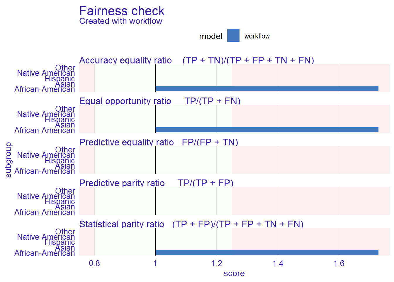

# Plot fairness object
  plot(fairness_object)

# Plot density of probability
  plot_density(fairness_object)

# Plot metric scores
  plot(metric_scores(fairness_object))

19 All the code

# namer::unname_chunks("13-bias_fairness.qmd")
# namer::name_chunks("13-bias_fairness.qmd")
options(scipen=99999)
metrics_combined <- metric_set(accuracy, recall, precision, f_meas, spec)

data_test %>%
      augment(x = fit_lr, type.predict = "response") %>%
      group_by(race) %>%
      metrics_combined(truth = reoffend_factor, estimate = .pred_class)
metrics_combined <- metric_set(
    equal_opportunity(race),
    equalized_odds(race),
    demographic_parity(race))

data_test %>%
    augment(x = fit_lr, type.predict = "response") %>%
    metrics_combined(truth = reoffend_factor, estimate = .pred_class)
# install.packages(pacman)
pacman::p_load(tidyverse,
               tidymodels,
               knitr,
               kableExtra,
               DataExplorer,
               visdat,
               naniar)
load(file = "www/data/data_compas.Rdata")
# install.packages(pacman)
pacman::p_load(tidyverse,
               tidymodels,
               knitr,
               kableExtra,
               DataExplorer,
               visdat,
               naniar)

rm(list=ls())
load(url(sprintf("https://docs.google.com/uc?id=%s&export=download",
                         "1gryEUVDd2qp9Gbgq8G0PDutK_YKKWWIk")))
table(data$race, useNA = "always") %>%
  kable(col.names = c("Race", "Frequency"))

data %>%
  ggplot(aes(x = fct_infreq(race))) + # fct_infreq(): reoder according to frequency
    geom_bar() + # create barplot
    geom_text(stat = "count", # add proportions
            aes(label = round((after_stat(count)) / sum(after_stat(count)), 2), 
                vjust = -0.5))
# Extract data with missing outcome
  data_missing_outcome <- data %>% filter(is.na(reoffend_factor))
  dim(data_missing_outcome)

# Omit individuals with missing outcome from data
  data <- data %>% drop_na(reoffend_factor) # ?drop_na
  dim(data)
  
# Split the data into training and test data
  data_split <- initial_split(data, prop = 0.80)
  data_split # Inspect

# Extract the two datasets
  data_train <- training(data_split)
  data_test <- testing(data_split) # Do not touch until the end!

  
# Define a recipe for preprocessing (taken from above)
  recipe_lr <- recipe(reoffend_factor ~ age + priors_count + race, data = data_train) %>%
    recipes::update_role(race, new_role = "id") # keep but don't use in model
  
# Define a model
  model_lr <- logistic_reg() %>% # logistic model
            set_engine("glm") %>% # define lm package/function
            set_mode("classification")
  
  
# Define a workflow
  workflow1 <- workflow() %>% # create empty workflow
    add_recipe(recipe_lr) %>% # add recipe
    add_model(model_lr) # add model  
  
# Fit the workflow (including recipe and model)
  fit_lr <- workflow1 %>% fit(data = data_train)


# Add prediction to training data and test data 
  data_train <- data_train %>% augment(x = fit_lr, type.predict = "response")
  data_test <- data_test %>% augment(x = fit_lr, type.predict = "response")
# Confusion matrix
  data_test %>%
      conf_mat(truth = reoffend_factor, 
               estimate = .pred_class) %>% 
  pluck("table") %>% t() %>% addmargins()


# Accuracy measures across groups
  metrics_combined <- metric_set(accuracy, recall, precision, f_meas, yardstick::spec) # Use several metrics
  
# Metrics for teh full testset (as benchmark)
  data_test %>%
    metrics_combined(truth = reoffend_factor, estimate = .pred_class)

# Across groups: Race
data_test %>%
  filter(race=="African-American"|race=="Caucasian") %>%
      group_by(race) %>%
      metrics_combined(truth = reoffend_factor, estimate = .pred_class) %>%
  pivot_wider(names_from = race, values_from = .estimate)
  
# Across groups: Race
data_test %>%
      group_by(sex) %>%
      metrics_combined(truth = reoffend_factor, estimate = .pred_class)%>%
  pivot_wider(names_from = sex, values_from = .estimate) 
# Visualize
  p1 <- data_test %>%
    metrics_combined(truth = reoffend_factor, estimate = .pred_class) %>%
    ggplot(aes(x = .metric, y = .estimate, color = .metric)) +
    geom_point(size = 3) +
    theme_minimal() + 
  theme(axis.text.x = element_text(angle = 45, hjust = 1)) +
  scale_y_continuous(breaks = seq(0, 1, by = 0.1),
                     limits = c(0,1))
  
  
  p2 <- data_test %>%
    filter(race=="African-American"|race=="Caucasian") %>%
      group_by(race) %>%
      metrics_combined(truth = reoffend_factor, estimate = .pred_class) %>%
    ungroup() %>%
    ggplot(aes(x = .metric, y = .estimate, color = race, group = race)) +
    geom_point(size = 3, position = position_dodge(width = 0.3)) +
    geom_line(position = position_dodge(width = 0.3))+
    theme_minimal() + 
    theme(axis.text.x = element_text(angle = 45, hjust = 1)) +
  scale_y_continuous(breaks = seq(0, 1, by = 0.1),
                     limits = c(0,1))
  
  
 # Across groups: sex
  p3 <- data_test %>%
      group_by(sex) %>%
      metrics_combined(truth = reoffend_factor, estimate = .pred_class) %>%
    ungroup() %>%
    ggplot(aes(x = .metric, y = .estimate, color = sex, group = sex)) +
    geom_point(size = 3, position = position_dodge(width = 0.3)) +
    geom_line(position = position_dodge(width = 0.3))+
    theme_minimal() + theme(axis.text.x = element_text(angle = 45, hjust = 1))+
  scale_y_continuous(breaks = seq(0, 1, by = 0.1),
                     limits = c(0,1)) 
  
library(patchwork)
  
 p1 + p2+ p3+
  plot_layout(axis_titles = "collect",
              design = "AAAAAA 
  BBBCCC")
# Specify metrics
  # Certain metrics are calculated for specific grouping variables
  # e.g., equal_opportunity(age_cat)
  metrics_combined <- metric_set(
                                      equal_opportunity(race),
                                      equalized_odds(race),
                                      demographic_parity(race),
                                      equal_opportunity(sex),
                                      equalized_odds(sex),
                                      demographic_parity(sex)) # Use several metrics



# Test data: Metrics
  data_test %>%
    filter(race=="African-American"|race=="Caucasian") %>%
    metrics_combined(truth = reoffend_factor, estimate = .pred_class) %>%
    ggplot(aes(x = .metric, y = .estimate, color = .by, group = .by)) +
    geom_point(size = 3, position = position_dodge(width = 0.3)) +
    geom_line(position = position_dodge(width = 0.3))+
    theme_minimal() +
  scale_y_continuous(breaks = seq(0, 1, by = 0.1),
                     limits = c(0,1)) 
  
# Define accuracy metrics
  metrics_combined <- metric_set(accuracy, recall, precision, f_meas, spec) # Use several metrics
  
# Metrics for full testset (as benchmark)
  data_test %>%
    metrics_combined(truth = reoffend_factor, estimate = .pred_class) %>%
    add_row(.metric = "FPR (1 - specificity)", 
            .estimator="binary", .estimate = 1-.$.estimate[5]) %>%
    add_row(.metric = "FNR (1 − recall/TPR)", 
            .estimator="binary", .estimate = 1-.$.estimate[2]) %>%
    add_row(.metric = "TNR (1 - FPR)", 
            .estimator="binary", .estimate = 1-.$.estimate[6]) %>%
    mutate(.metric = recode(.metric,
                            "recall" = "recall/TPR"))
# Accuracy measures across groups
  metrics_combined <- metric_set(accuracy, recall, precision, f_meas, spec)
  
# Metrics for thh full testset (as benchmark)
metrics_African_American <- 
    data_test %>%
    filter(race=="African-American") %>%
    metrics_combined(truth = reoffend_factor, estimate = .pred_class) %>%
    add_row(.metric = "FPR (1 - specificity)", 
            .estimator="binary", .estimate = 1-.$.estimate[5]) %>%
    add_row(.metric = "FNR (1 − recall/TPR)", 
            .estimator="binary", .estimate = 1-.$.estimate[2]) %>%
    add_row(.metric = "TNR (1 - FPR)", 
            .estimator="binary", .estimate = 1-.$.estimate[6]) %>%
    mutate(.metric = recode(.metric,
                            "recall" = "recall/TPR")) %>%
  rename("African_American" = ".estimate")

metrics_Caucasian <- 
    data_test %>%
    filter(race=="Caucasian") %>%
    metrics_combined(truth = reoffend_factor, estimate = .pred_class) %>%
    add_row(.metric = "FPR (1 - specificity)", 
            .estimator="binary", .estimate = 1-.$.estimate[5]) %>%
    add_row(.metric = "FNR (1 − recall/TPR)", 
            .estimator="binary", .estimate = 1-.$.estimate[2]) %>%
    add_row(.metric = "TNR (1 - FPR)", 
            .estimator="binary", .estimate = 1-.$.estimate[6]) %>%
    mutate(.metric = recode(.metric,
                            "recall" = "recall/TPR")) %>%
  rename("Caucasian" = ".estimate")

metrics_all <- 
  bind_cols(metrics_African_American %>% select(-.estimator),
            metrics_Caucasian %>% select(-.estimator, -.metric))

metrics_all
table(data$race)
table(data$sex)
table(data$age_cat)
library(ggplot2)
library(patchwork)
p1 <- ggplot(data = data, 
             aes(x = decile_score)) + 
  geom_histogram(binwidth = 1) +
  scale_x_continuous(breaks = 0:10) + 
  theme_light()
p2 <- ggplot(data = data, 
             aes(x = decile_score)) + 
  geom_histogram(binwidth = 1) +
  scale_x_continuous(breaks = 0:10) + 
  theme_light() +
  facet_wrap(~race)


p1+p2
data$.pred_class_compas <- factor(ifelse(data$decile_score > 5, "yes", "no"))
table(data$decile_score, data$.pred_class_compas)
# Confusion matrix
  data %>%
      conf_mat(truth = reoffend_factor, 
               estimate = .pred_class_compas) %>% 
  pluck("table") %>% t() %>% addmargins()


# Accuracy measures across groups
  metrics_combined <- metric_set(accuracy, recall, precision, f_meas, spec)
  
# Metrics for teh full testset (as benchmark)
  data %>%
    metrics_combined(truth = reoffend_factor, estimate = .pred_class_compas)


# Across groups: Race
data %>%
  filter(race=="African-American"|race=="Caucasian") %>%
      group_by(race) %>%
      metrics_combined(truth = reoffend_factor, estimate = .pred_class_compas) %>%
  pivot_wider(names_from = race, values_from = .estimate)
# Visualize
  p1 <- data %>%
    metrics_combined(truth = reoffend_factor, estimate = .pred_class_compas) %>%
    ggplot(aes(x = .metric, y = .estimate, color = .metric)) +
    geom_point(size = 3) +
    theme_minimal() + 
  theme(axis.text.x = element_text(angle = 45, hjust = 1)) +
  scale_y_continuous(breaks = seq(0, 1, by = 0.1),
                     limits = c(0,1))
  
  
  p2 <- data %>%
    filter(race=="African-American"|race=="Caucasian") %>%
      group_by(race) %>%
      metrics_combined(truth = reoffend_factor, estimate = .pred_class_compas) %>%
    ungroup() %>%
    ggplot(aes(x = .metric, y = .estimate, color = race, group = race)) +
    geom_point(size = 3, position = position_dodge(width = 0.3)) +
    geom_line(position = position_dodge(width = 0.3))+
    theme_minimal() + 
    theme(axis.text.x = element_text(angle = 45, hjust = 1)) +
  scale_y_continuous(breaks = seq(0, 1, by = 0.1),
                     limits = c(0,1))
  
  
 # Across groups: sex
  p3 <- data %>%
      group_by(sex) %>%
      metrics_combined(truth = reoffend_factor, estimate = .pred_class_compas) %>%
    ungroup() %>%
    ggplot(aes(x = .metric, y = .estimate, color = sex, group = sex)) +
    geom_point(size = 3, position = position_dodge(width = 0.3)) +
    geom_line(position = position_dodge(width = 0.3))+
    theme_minimal() + theme(axis.text.x = element_text(angle = 45, hjust = 1))+
  scale_y_continuous(breaks = seq(0, 1, by = 0.1),
                     limits = c(0,1)) 
  
library(patchwork)
  
 p1 + p2+ p3+
  plot_layout(axis_titles = "collect",
              design = "AAAAAA 
  BBBCCC")
# Specify metrics
  # Certain metrics are calculated for specific grouping variables
  # e.g., equal_opportunity(age_cat)
  metrics_combined <- metric_set(
                                      equal_opportunity(race),
                                      equalized_odds(race),
                                      demographic_parity(race),
                                      equal_opportunity(sex),
                                      equalized_odds(sex),
                                      demographic_parity(sex)) # Use several metrics



# Test data: Metrics
  data %>%
    filter(race=="African-American"|race=="Caucasian") %>%
    metrics_combined(truth = reoffend_factor, estimate = .pred_class_compas) %>%
    ggplot(aes(x = .metric, y = .estimate, color = .by, group = .by)) +
    geom_point(size = 3, position = position_dodge(width = 0.3)) +
    geom_line(position = position_dodge(width = 0.3))+
    theme_minimal() +
  scale_y_continuous(breaks = seq(0, 1, by = 0.1),
                     limits = c(0,1)) 
  
# Accuracy measures across groups
  metrics_combined <- metric_set(accuracy, recall, precision, f_meas, spec)
  
# Metrics for the full testset (as benchmark)
metrics_African_American <- 
    data %>%
    filter(race=="African-American") %>%
    metrics_combined(truth = reoffend_factor, estimate = .pred_class_compas) %>%
    add_row(.metric = "FPR (1 - specificity)", .estimator="binary", .estimate = 1-.$.estimate[5]) %>%
    add_row(.metric = "FNR (1 − recall/TPR)", .estimator="binary", .estimate = 1-.$.estimate[2]) %>%
    add_row(.metric = "TNR (1 - FPR)", .estimator="binary", .estimate = 1-.$.estimate[6]) %>%
    mutate(.metric = recode(.metric,
                            "recall" = "recall/TPR")) %>%
  rename("African_American" = ".estimate")

metrics_Caucasian <- 
    data %>%
    filter(race=="Caucasian") %>%
    metrics_combined(truth = reoffend_factor, estimate = .pred_class_compas) %>%
    add_row(.metric = "FPR (1 - specificity)", .estimator="binary", .estimate = 1-.$.estimate[5]) %>%
    add_row(.metric = "FNR (1 − recall/TPR)", .estimator="binary", .estimate = 1-.$.estimate[2]) %>%
    add_row(.metric = "TNR (1 - FPR)", .estimator="binary", .estimate = 1-.$.estimate[6]) %>%
    mutate(.metric = recode(.metric,
                            "recall" = "recall/TPR")) %>%
  rename("Caucasian" = ".estimate")

metrics_all <- 
  bind_cols(metrics_African_American %>% select(-.estimator),
            metrics_Caucasian %>% select(-.estimator, -.metric))

metrics_all
# install.packages(pacman)
pacman::p_load(tidyverse,
               tidymodels,
               knitr,
               kableExtra,
               DataExplorer,
               visdat,
               naniar)
load(file = "www/data/data_compas.Rdata")
# install.packages(pacman)
pacman::p_load(tidyverse,
               tidymodels,
               knitr,
               kableExtra,
               DataExplorer,
               visdat,
               naniar)

rm(list=ls())
load(url(sprintf("https://docs.google.com/uc?id=%s&export=download",
                         "1gryEUVDd2qp9Gbgq8G0PDutK_YKKWWIk")))
library(DALEX)
library(DALEXtra)
library(fairmodels)

  data <- data %>% select(-id, -name, -decile_score, -reoffend, -age, -compas_screening_date) |> filter(race=="African-American"|race=="Caucasian")


# Extract data with missing outcome
  data_missing_outcome <- data %>% filter(is.na(reoffend_factor))
  dim(data_missing_outcome)

# Omit individuals with missing outcome from data
  data <- data %>% drop_na(reoffend_factor) # ?drop_na
  dim(data)
  
# Split the data into training and test data
  data_split <- initial_split(data, prop = 0.80)
  data_split # Inspect

# Extract the two datasets
  data_train <- training(data_split)
  data_test <- testing(data_split) # Do not touch until the end!

  
# Define a recipe for preprocessing (taken from above)
  recipe_lr <- recipe(reoffend_factor ~ ., data = data_train) %>%
    recipes::update_role(race, new_role = "id")
  
# Define a model
  model_lr <- logistic_reg() %>% # logistic model
            set_engine("glm") %>% # define lm package/function
            set_mode("classification")
  
  
# Define a workflow
  workflow1 <- workflow() %>% # create empty workflow
    add_recipe(recipe_lr) %>% # add recipe
    add_model(model_lr) # add model  
  
# Fit the workflow (including recipe and model)
  fit_lr <- workflow1 %>% fit(data = data_train)





# save out the protected variable ("Race") for later reference for Fairness checking
  protected <- bake(recipe_lr |> prep(), new_data = data_train) |> select(race) |> pull()

# create the DALEX-based explainer object, which draws upon the fitted Tidymodels Workflow, the training data and our predicted variable

  model_explainer <- 
    DALEXtra::explain_tidymodels(
      fit_lr,
      data    = data_train |> select(-reoffend_factor),
      y       = as.numeric(data_train$reoffend_factor),
      verbose = FALSE
  )

# Display model performance
  model_performance(model_explainer)

# Use explainer object & perform a fairness check
fairness_object <- fairness_check(model_explainer,
                          protected  = protected,
                          privileged = "Caucasian",
                          colorize = TRUE)
# Print fairness object
  print(fairness_object)

# Plot fairness object
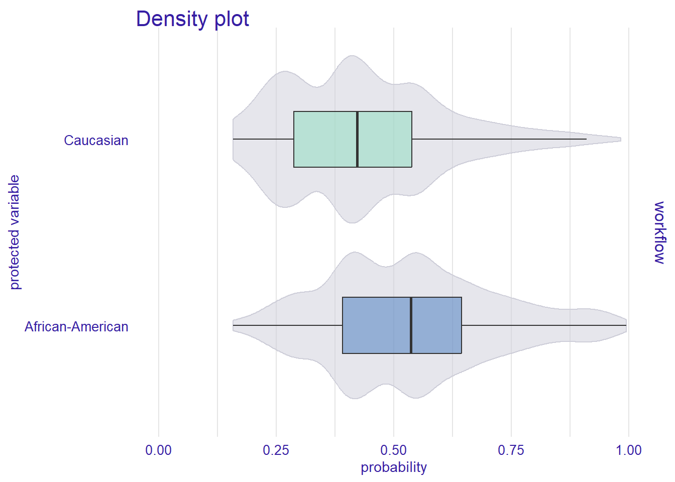
  plot(fairness_object)

# Plot density of probability
  plot_density(fairness_object)

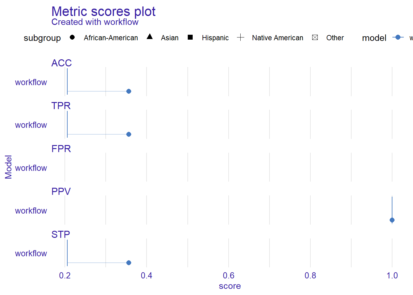
# Plot metric scores
  plot(metric_scores(fairness_object))
labs = knitr::all_labels()
ignore_chunks <- labs[str_detect(labs, "setup|solution|get-labels|load-local-data")]
labs = setdiff(labs, ignore_chunks)

References

AlgorithmWatch. 2019. “Atlas of Automation Automated Decision-Making and Participation in Germany.”

Angwin, Julia, Jeff Larson, Lauren Kirchner, and Surya Mattu. 2016. “Machine Bias.” https://www.propublica.org/article/machine-bias-risk-assessments-in-criminal-sentencing.

Barocas, Solon, and Andrew D Selbst. 2016. “Big Data’s Disparate Impact.” California Law Review 104: 671.

Berk, Richard, Hoda Heidari, Shahin Jabbari, Michael Kearns, and Aaron Roth. 2021. “Fairness in Criminal Justice Risk Assessments: The State of the Art.” Sociological Methods & Research 50 (1): 3–44.

Corbett-Davies, Sam, Emma Pierson, Avi Feller, Sharad Goel, and Aziz Huq. 2017. “Algorithmic Decision Making and the Cost of Fairness.” In Proceedings of the 23rd ACM SIGKDD International Conference on Knowledge Discovery and Data Mining. ACM.

Dressel, Julia, and Hany Farid. 2018. “The Accuracy, Fairness, and Limits of Predicting Recidivism.” Science Advances 4 (1): eaao5580.

Dwork, Cynthia, Moritz Hardt, Toniann Pitassi, Omer Reingold, and Richard Zemel. 2012. “Fairness Through Awareness.” In Proceedings of the 3rd Innovations in Theoretical Computer Science Conference, 214–26. Association for Computing Machinery.

Grgic-Hlaca, Nina, Muhammad Bilal Zafar, Krishna P Gummadi, and Adrian Weller. 2016. “The Case for Process Fairness in Learning: Feature Selection for Fair Decision Making.” In NIPS Symposium on Machine Learning and the Law, 1:11. mlandthelaw.org.

Hardt, Moritz, Eric Price, and Nathan Srebro. 2016. “Equality of Opportunity in Supervised Learning.” Advances in Neural Information Processing Systems.

James, Gareth, Daniela Witten, Trevor Hastie, and Robert Tibshirani. 2013. An Introduction to Statistical Learning: With Applications in R. Springer.

Kamiran, Faisal, and Indrė Žliobaitė. 2013. “Explainable and Non-Explainable Discrimination in Classification.” In Discrimination and Privacy in the Information Society: Data Mining and Profiling in Large Databases, edited by Bart Custers, Toon Calders, Bart Schermer, and Tal Zarsky, 155–70. Springer Berlin Heidelberg.

Kleinberg, Jon, Sendhil Mullainathan, and Manish Raghavan. 2016. “Inherent Trade-Offs in the Fair Determination of Risk Scores.” arXiv [Cs.LG].

Kusner, Matt J, Joshua Loftus, Chris Russell, and Ricardo Silva. 2017. “Counterfactual Fairness.” Advances in Neural Information Processing Systems 30.

Lee, Claire S, Jeremy Du, and Michael Guerzhoy. 2020. “Auditing the COMPAS Recidivism Risk Assessment Tool: Predictive Modelling and Algorithmic Fairness in CS1.” In Proceedings of the 2020 ACM Conference on Innovation and Technology in Computer Science Education, 535–36. Association for Computing Machinery.

Mehrabi, Ninareh, Fred Morstatter, Nripsuta Saxena, Kristina Lerman, and Aram Galstyan. 2021. “A Survey on Bias and Fairness in Machine Learning.” ACM Comput. Surv. 54 (6): 1–35.

Osoba, Osonde, and William Welser IV. 2017. “An Intelligence in Our Image.” Santa Mônica: RAND Corporation.

Rodolfa, Kit T, Pedro Saleiro, and Rayid Ghani. 2020. “Bias and Fairness.” In Big Data and Social Science, 281–312. Chapman; Hall/CRC.

Saleiro, Pedro, Benedict Kuester, Loren Hinkson, Jesse London, Abby Stevens, Ari Anisfeld, Kit T Rodolfa, and Rayid Ghani. 2018. “Aequitas: A Bias and Fairness Audit Toolkit.” arXiv [Cs.LG].

Saxena, Nripsuta Ani. 2019. “Perceptions of Fairness.” In Proceedings of the 2019 AAAI/ACM Conference on AI, Ethics, and Society, 537–38. Association for Computing Machinery.

Saxena, Nripsuta Ani, Karen Huang, Evan DeFilippis, Goran Radanovic, David C Parkes, and Yang Liu. 2019. “How Do Fairness Definitions Fare? Examining Public Attitudes Towards Algorithmic Definitions of Fairness.” In Proceedings of the 2019 AAAI/ACM Conference on AI, Ethics, and Society, 99–106. Association for Computing Machinery.

Verma, Sahil, and Julia Rubin. 2018. “Fairness Definitions Explained.” In Proceedings of the International Workshop on Software Fairness, 1–7. Association for Computing Machinery.

Footnotes

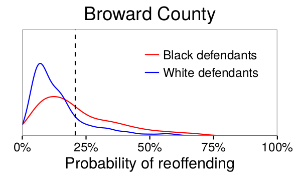
“The reason for these disparities is that white and black defendants in Broward County have different distributions of risk, \(p_{Y|X}\), as shown in Figure 1. In particular, a greater fraction of black defendants have relatively high risk scores, in part because black defendants are more likely to have prior arrests, which is a strong indicator of reoffending. Importantly, while an algorithm designer can choose different decision rules based on these risk scores, the algorithm cannot alter the risk scores themselves, which reflect underlying features of the population of Broward County.” (Corbett-Davies et al. 2017, 803)↩︎
https://go.volarisgroup.com/rs/430-MBX-989/images/ProPublica_Commentary_Final_070616.pdf↩︎
The False Positive Rate measures the proportion of negative instances incorrectly classified as positive.Interpretation: For COMPAS, this reflects how often individuals who do not reoffend are incorrectly predicted to reoffend. The False Negative Rate measures the proportion of positive instances incorrectly classified as negative. Interpretation: This reflects how often individuals who will reoffend are incorrectly predicted not to reoffend. The False Discovery Rate measures the proportion of positive predictions that are incorrect (false positives). Interpretation: This reflects how often predictions of reoffending turn out to be wrong.↩︎
FPR = 45%; FNR = 28%; FDR = 69.4%;↩︎
Reason: On average females work fewer hours than males per week↩︎
Reverse discrimination is a term often used to describe a situation in which policies or actions designed to correct historical or systemic discrimination against certain groups (e.g., racial minorities, women) end up discriminating against individuals from historically privileged groups (e.g., white people, men). The term suggests that measures taken to promote affirmative action, diversity, or equal opportunity might inadvertently lead to unfair treatment of members of groups who are not the intended beneficiaries of those policies.↩︎
Example 1: Many companies have policies that prefer younger candidates, believing they are more adaptable, tech-savvy, or able to work long hours. This could be seen as explainable discrimination because it is based on the assumption that age correlates with specific skills or energy levels. Example 2: Some armed forces have gender-specific physical standards for recruitment, where men and women are assessed differently based on physical performance criteria. Example 3: Many businesses offer senior discounts, where older individuals (usually over a certain age, like 65 or 70) receive reduced prices on products or services because they earn less.↩︎
= Antidiskriminierungsgesetz↩︎
= GDPR = General Data Protection Regulation↩︎
e.g., COMPAS, where prior arrests and friend/family arrests were used as proxy variables to measure level of “riskiness” or “crime”↩︎
e.g., forgetting the predictor of ‘prior offenses’↩︎
e.g. ImageNet: bias towards Western cultures (see Figure 3 and 4 in Mehrabi et al. 2021)↩︎
i.e., any general assumptions about subgroups within the population can result in aggregation bias; see also Simpson’s Paradox – Simpson’s Paradox can reveal hidden biases within the data that might not be apparent when analyzing the dataset as a whole. When data from different groups are aggregated, it can mask underlying trends that are only visible when the data is segmented. This is particularly important in machine learning, where models trained on aggregated data might inadvertently perpetuate or even amplify these hidden biases, leading to unfair or biased outcomes. Understanding Simpson’s Paradox is crucial for ensuring fairness across different subgroups within the data. Machine learning models need to perform equitably across various demographics, such as gender, race, age, etc. – and the Modifiable Areal Unit Problem – A source of statistical bias that can significantly affect the analysis of geographical data. It arises when the results of an analysis change based on the scale or the zoning (i.e., the way in which areas are delineated and aggregated) of the spatial units used in the study.↩︎
Researchers analyzing temporal data must use longitudinal analysis to track cohorts over time to learn their behavior. Instead, temporal data is often modeled using cross-sectional analysis, which combines diverse cohorts at a single time point; e.g., comment length on reddit decreased over time, however, did increase when aggregated according to cohorts↩︎
e.g. only considering links (not content/behavior) in the network could favor low-degree nodes↩︎
e.g., optimization functions, regularizations, choices in applying regression models on the data as a whole or considering subgroups, and the general use of statistically biased estimators in algorithms↩︎
e.g., Presentation Bias is a result of how information is presented; Ranking Bias describes the idea that top-ranked results are the most relevant and important will result in attraction of more clicks than others. This bias affects search engines/crowdsourcing applications.↩︎
e.g., A voice recognition system trained primarily on native English speakers may struggle with non-native accents over time, reflecting a cultural and linguistic shift in user demographics.↩︎
e.g., use of inappropriate and disproportionate benchmarks for evaluation of applications such as Adience and IJB-A benchmarks that were used in the evaluation of facial recognition systems that were biased toward skin color and gender↩︎
e.g., 2018 image search result where searching for women CEOs ultimately resulted in fewer female CEO images due to the fact that only 5% of Fortune 500 CEOs were women-which would cause the search results to be biased towards male CEOs (reflects reality but do we want that)↩︎
e.g., when building a model that predicts whether users share fake news↩︎
e.g., enthusiastic supporters of candidate are more likely to complete the poll that should measure popularity of their candidate, which is later used to predict who is a supporter↩︎
e.g., we want to rate or review an item with a low score, but are influenced by other high ratings (Q: Can you think of an example?)↩︎
e.g., differences in emoji representations among platforms can result in different reactions and behavior from people and sometimes even leading to communication errors↩︎
e.g., Twitter used different hashtags to talk about politics in 2018 than in 2024↩︎
e.g., differences in use of language across different gender and age groups↩︎
Definition 5 in Mehrabi et al. (2021)↩︎
In the context of fair machine learning, redundant encoding refers to the practice of introducing extra features (or encoding attributes) into the model either to account for sensitive attributes like race, gender, age, etc., in ways that help ensure fairness or to remove or mask the influence. Importantly, ML models can easily pick up correlates of protected attributes, e.g., even if you remove race from the data, variables like zip code, education level, or income might still act as proxies for race.↩︎
“Unaware models” cannot model different mechanisms across groups, e.g., if a healthcare model ignores sex as a feature, it might fail to account for the different ways diseases manifest across men and women. This can result in a one-size-fits-all model that is less effective for all groups and fails to capture the true causal mechanisms driving the outcomes.↩︎
Definition 4 in Mehrabi et al. (2021)↩︎
Definition 3 in Mehrabi et al. (2021)↩︎
e.g., if a hiring algorithm produces an acceptance rate of 30% for both women (protected group) and men (unprotected group), the system satisfies demographic parity.↩︎
A biased decision-maker could intentionally reject highly qualified individuals from a protected group while still maintaining the required acceptance rate by accepting less qualified candidates instead. This reinforces stereotypes, e.g., “Women in tech are less competent” if the accepted women are underqualified, and may lead to a self-fullfilling prophecy.↩︎
e.g., a hiring algorithm should ensure equal acceptance rates across genders, conditional on job-relevant qualifications like years of experience or certifications.↩︎
FDR = false discovery rate; Predictive parity ensures that the proportion of false positives among all predicted positives is the same for all groups.↩︎
FOR = false omission rate; Equal \(FOR_{g}\) ensures that the likelihood of missing a true positive (= false negative) is the same across groups. This is particularly relevant in situations where false negatives carry serious consequences (e.g., misdiagnosing a medical condition).↩︎
Sufficiency ensures that the model’s predictions are equally reliable across all groups, whether considering positively predicted outcomes (via \(FDR_g\)) or negatively predicted outcomes (via \(FOR_g\)).↩︎
These metrics (predictive parity, \(FOR_{g}\), and sufficiency) focus on the reliability of the model’s predictions—ensuring that decisions based on those predictions are fair for different groups. This aligns with the interests of decision-makers, who need confidence that the model does not disproportionately harm or benefit certain groups in its predictions.↩︎
Predictive equality ensures that individuals in different groups have the same chance of being falsely labeled as “positive” when they shouldn’t be. This is particularly important when a false positive leads to unnecessary burden or harm (e.g., being flagged as a potential fraudster or being falsely diagnosed with a disease).↩︎
Equal opportunity ensures that individuals in different groups have the same chance of being correctly identified for a positive outcome. This is especially critical when a false negative denies someone access to beneficial outcomes (e.g., not getting a loan when qualified or missing a scholarship opportunity).↩︎
Equal Opportunity (Definition 2 in Mehrabi et al. (2021)) (Hardt, Price, and Srebro 2016): probability of a person in a positive class being assigned to a positive outcome should be equal for both protected and unprotected (female and male) group members (Verma and Rubin 2018), i.e., the equal opportunity definition states that the protected and unprotected groups should have equal true positive rates ↩︎
Equalized odds is a more stringent fairness criterion because it balances fairness for individuals in different groups for both types of errors. Equalized Odds (Definition 1 in Mehrabi et al. (2021)) (Hardt, Price, and Srebro 2016): probability of a person in the positive (true) class being correctly predicted a positive outcome and the probability of a person in a negative (true) class being incorrectly predicted a positive outcome should both be the same for the protected and unprotected group members (Verma and Rubin 2018), i.e, protected and unprotected groups should have equal rates for true positives and false positives↩︎
This focus on errors aligns with the experiences of individuals who interact with the system, making these metrics particularly relevant from the perspective of fairness for the affected.↩︎
Overall accuracy equality ensures that the model performs with the same overall level of accuracy for each group. For example, if a model has a 90% accuracy for one group, it should also have 90% accuracy for all other groups.↩︎
Treatment equality ensures that the ratio of false positives to false negatives is equal across groups. This means that one group is not unfairly burdened by more false positives while another group suffers more from false negatives.↩︎
Treatment Equality (Definition 6 in Mehrabi et al. (2021)): “Treatment equality is achieved when the ratio of false negatives and false positives is the same for both protected group categories” (Berk et al. 2021).↩︎
Measures help identify whether one group is experiencing disproportionately more false positives or false discoveries compared to another group. A higher disparity indicates that one group is facing a higher error rate than the baseline group, which could suggest unfair treatment or bias in the model’s predictions.↩︎
The False Discovery Rate (FDR) disparity is a measure comparing the false discovery rate for a specific group, e.g., protected group like women or minorities, with the false discovery rate for a baseline group, e.g., unprotected group like men or majority group. ↩︎
False positive rate↩︎
\(\tau\): A pre-defined threshold value that represents the acceptable level of disparity. Typically, this could be something like 0.8 or 1.25, depending on the fairness standard.↩︎
Conditional use accuracy equality means that a model’s accuracy should be the same for all protected groups when it predicts the same probability of an outcome for individuals within those groups. Suppose a model predicts the likelihood of recidivism (reoffending) for individuals. If two individuals from different racial groups both receive a predicted probability of 0.8 for recidivism, conditional use accuracy equality means that both individuals’ predictions should be equally accurate, regardless of their race – i.e., if the predicted outcome is positive (reoffending), the model should be equally likely to correctly predict reoffending for both individuals.↩︎
See also Kleinberg, Mullainathan, and Raghavan (2016).↩︎
\(F_1 = 2 \times \frac{\text{Precision} \times \text{Recall}}{\text{Precision} + \text{Recall}}\)↩︎
Satisfied when a model’s predictions have the same true positive rate TPR (or false negative rates FNR) across protected groups. A value of 0 indicates parity across groups. \(TPR = 1 - FNR\) and vice versa.↩︎
Satisfied when a model’s predictions have the same false positive, true positive, false negative, and true negative rates across protected groups. A value of 0 indicates parity across groups.↩︎
Satisfied when a model’s predictions have the same predicted positive rate across groups. A value of 0 indicates parity across groups.↩︎
Eselsbrücke: Sensitivity (recall) → Sniffer: Finds as many positives as possible, even if there are some false positives. Specificity → Selective: Focuses on correctly identifying negatives without false positives.↩︎
The results look pretty bad for race.↩︎

1 Overview

2 Automated Decision-Making (ADM)

3 Databases on ADM systems

4 The COMPAS Case I

5 The COMPAS Case II

6 The COMPAS Case III

7 The COMPAS Case IV

8 The COMPAS Case V: Error rates

9 Examples of discrimination & bias: Exercise

10 Fairness and Automated Decision-Making

11 Discrimination & protected attributes

11.1 Legal discrimination definitions (Barocas and Selbst 2016)

11.2 Explainable Discrimination

11.3 Unexplainable Discrimination & Sources

11.4 Protected attributes (U.S.)

11.5 Protected attributes (Germany/Europe)

12 Biases

12.1 Biases in a feed-back loop

12.2 Exercise: Biases in a feed-back loop

12.3 Biases: Data to Algorithm

12.4 Biases: Algorithm to User

12.5 Biases: User to Data

12.6 Exercise: Biases

13 Algorithmic fairness definitions

13.1 Fairness definitions (1)

13.2 Fairness definitions (2): Equality of Treatment

13.3 Fairness definitions (2): Equality of Outcomes

13.4 Fairness definitions (4): overview

13.5 Fairness definitions (5): Equality of Errors

13.6 Fairness definitions (6): Sufficiency

13.7 Fairness definitions (7): Equalized Odds

13.8 Fairness definitions (8): Accuracy Equality

13.9 Fairness definitions (9): Group disparity measures

13.10 Fairness Trade-offs: Impossibility of Fairness

14 Tidymodels

14.1 Tidymodels: Accuracy equality (1)

14.2 Tidymodels: Accuracy equality (2)

14.3 Tidymodels: Fairness (1)

15 Lab: Assessing fairness in R

15.1 Estimate model

15.1.1 Accuracy across groups

15.1.2 Fairness across groups

15.1.3 More metrics (fairness)

16 Exercise/Homework: Fairness

17 Lab: Northpointe Compas score fairness

18 Lab: Using fairmodels package (experimental!)

19 All the code

References

Footnotes

18 Lab: Using `fairmodels` package (experimental!)