# load and install packages if neccessary
if(!require("rvest")) {install.packages("rvest"); library("rvest")}
if(!require("xml2")) {install.packages("xml2"); library("xml2")}
if(!require("tidytext")) {install.packages("tidytext"); library("tidytext")}
if(!require("tibble")) {install.packages("tibble"); library("tibble")}
if(!require("dplyr")) {install.packages("dplyr"); library("dplyr")}Text classification
Chapter last updated: 10 Februar 2025
Learning outcomes/objective: Learn…
- …about basic concepts of Natural Language Processing (NLP)
- …become familiar with a typical R-tidymodels-workflow for text analysis
- …overview machine learning approaches for text data (supervised & unsupervised)
- Lab: Supervised text classification with tidymodels.
Sources: Camille Landesvatter’s topic model lecture, Original material & see references; Tuning text models
1 Text as Data
- Many sources of text data for social scientists
- open ended survey responses, social media data, interview transcripts, news articles, official documents (public records, etc.), research publications, etc.
- even if data of interest not in textual form (yet)
- speech recognition, text recognition, machine translation etc.
- “Past”: text data often ignored (by quants), selectively read, anecdotally used or manually labeled by researchers
- Today: wide variety of text analytically methods (supervised + unsupervised) and increasing adoption of these methods by social scientists (Wilkerson and Casas 2017)
2 Language in NLP
- corpus: a collection of documents
- documents: single tweets, single statements, single text files, etc.
- tokenization: “the process of splitting text into tokens” (Silge and Robinson 2017), further refers to defining the unit of analysis, i.e., tokens = single words, sequences of words or entire sentences
- bag of words (method): approach where all tokens are put together in a “bag” without considering their order (alternatively: bigrams/word pairs, word embeddings)
- possible issues with a simple bag-of-word: “I’m not happy and I don’t like it!”
- stop words: very common but uninformative terms (really?) such as “the”, “and”, “they”, etc.
- document-term/feature matrix (DTM/DFM): common format to store text data (examples later)
3 (R-)Workflow for Text Analysis
- Data collection (“Obtaining Text”*)
- Data manipulation / Corpus pre-processing (“From Text to Data”*)
- Vectorization: Turning Text into a Matrix (DTM/DFM1) (“From Text to Data”*)
- Analysis (“Quantitative Analysis of Text”*)
- Validation and Model Selection (“Evaluating Performance”2)
- Visualization and Model Interpretation
3.1 Data collection
- use existing corpora
- collect new corpora
- electronic sources: application user interfaces (APIs, e.g. Facebook, Twitter), web scraping, wikipedia, transcripts of all german electoral programs
- undigitized text, e.g. scans of documents
- data from interviews, surveys and/or experiments (speech → text)
- consider relevant applications to turn your data into text format (speech-to-text recognition, pdf-to-text, OCR, Mechanical Turk and Crowdflower)
4 Data manipulation
4.1 Data manipulation: Basics (1)
- text data is different from “structured” data (e.g., a set of rows and columns)
- most often not “clean” but rather messy
- shortcuts, dialect, incorrect grammar, missing words, spelling issues, ambiguous language, humor
- web context: emojis, # (twitter), etc.
- Preprocessing much more important & crucial determinant of successful text analysis!
4.2 Data manipulation: Basics (2)
Common steps in pre-processing text data:
stemming (removal of word suffixes), e.g., computation, computational, computer \(\rightarrow\) compute
lemmatisation (reduce a term to its lemma, i.e., its base form), e.g., “better” \(\rightarrow\) “good”
transformation to lower cases
removal of punctuation (e.g., ,;.-) / numbers / white spaces / URLs / stopwords / very infrequent words
\(\rightarrow\) Always choose your preprocessing steps carefully!
- e.g., removing punctuation: “I enjoy: eating, my cat and leaving out commas” vs. “I enjoy: eating my cat and leaving out commas”
Unit of analysis?! (sentence vs. unigram vs. bigram etc.)
4.3 Data manipulation: Basics (3)
In principle, all those transformations can be achieved by using base R
Other packages however provide ready-to-apply functions, such as {tidytext}, {tm} or {quanteda}
Important
- transform data to corpus object or tidy text object (examples on the next slides) or use tidymodels step functions
4.4 Data manipulation: Tidytext Example (1) (skipped)
Pre-processing with tidytext requires your data to be stored in a tidy text object.
Q: What are main characteristics of a tidy text dataset?
- one-token-per-row
- “long format”
First, we have to retrieve some data. In keeping with today’s session, we will use data from Wikipedias entry on Natural Language Processing.
# import wikipedia entry on Natural Language Processing, parsed by paragraph
text <- read_html("https://en.wikipedia.org/wiki/Natural_language_processing#Text_and_speech_processing") %>%
  html_nodes("#content p")%>%
  html_text()

# we decide to keep only paragraph 1 and 2
text<-text[1:2]

text
[1] "Natural language processing (NLP) is a subfield of computer science and especially artificial intelligence. It is primarily concerned with providing computers with the ability to process data encoded in natural language and is thus closely related to information retrieval, knowledge representation and computational linguistics, a subfield of linguistics. Typically data is collected in text corpora, using either rule-based, statistical or neural-based approaches in machine learning and deep learning.\n"
[2] "Major tasks in natural language processing are speech recognition, text classification, natural-language understanding, and natural-language generation.\n" In order to turn this data into a tidy text dataset, we first need to put it into a data frame (or tibble).
# put character vector into a data frame
# also add information that data comes from the wiki entry on NLP and from which paragraphs
wiki_df <- tibble(topic=c("NLP"), paragraph=1:2, text=text)

str(wiki_df)
tibble [2 × 3] (S3: tbl_df/tbl/data.frame)
$ topic : chr [1:2] "NLP" "NLP"
$ paragraph: int [1:2] 1 2
$ text : chr [1:2] "Natural language processing (NLP) is a subfield of computer science and especially artificial intelligence. It "| __truncated__ "Major tasks in natural language processing are speech recognition, text classification, natural-language unders"| __truncated__Q: Describe the above dataset. How many variables and observations are there? What do the variables display?
Now, by using the unnest_tokens() function from tidytext we transform this data to a tidy text format.
Q: How does our dataset change after tokenization and removing stopwords? How many observations do we now have? And what does the paragraph variable identify/store?
Q: Also, have a closer look at the single words. Do you notice anything else that has changed, e.g., is something missing from the original text?
tibble [59 × 3] (S3: tbl_df/tbl/data.frame)
 $ topic    : chr [1:59] "NLP" "NLP" "NLP" "NLP" ...
 $ paragraph: int [1:59] 1 1 1 1 1 1 1 1 1 1 ...
$ word : chr [1:59] "natural" "language" "processing" "nlp" ... [1] "natural" "language" "processing" "nlp" "subfield"
[6] "computer" "science" "artificial" "intelligence" "primarily"
[11] "concerned" "providing" "computers" "ability" "process" 4.5 Data manipulation: Tidytext Example (2) (skipped)
“Pros” and “Cons”:
tidytext removes punctuation and makes all terms lowercase automatically (see above)
all other transformations need some dealing with regular expressions
- example to remove white space with tidytext (s+ describes a blank space):
[1] "Naturallanguageprocessing(NLP)isasubfieldofcomputerscienceandespeciallyartificialintelligence.Itisprimarilyconcernedwithprovidingcomputerswiththeabilitytoprocessdataencodedinnaturallanguageandisthuscloselyrelatedtoinformationretrieval,knowledgerepresentationandcomputationallinguistics,asubfieldoflinguistics.Typicallydataiscollectedintextcorpora,usingeitherrule-based,statisticalorneural-basedapproachesinmachinelearninganddeeplearning."
[2] "Majortasksinnaturallanguageprocessingarespeechrecognition,textclassification,natural-languageunderstanding,andnatural-languagegeneration." - \(\rightarrow\) consider alternative packages (e.g., tm, quanteda)
Example: tm package
- input: corpus not tidytext object
- What is a corpus in R? \(\rightarrow\) group of documents with associated metadata
# Load the tm package
library(tm)

# Clean corpus
corpus_clean <- VCorpus(VectorSource(wiki_df$text)) %>%
  tm_map(removePunctuation, preserve_intra_word_dashes = TRUE) %>%
  tm_map(removeNumbers) %>%
  tm_map(content_transformer(tolower)) %>%
  tm_map(removeWords, words = c(stopwords("en"))) %>%
  tm_map(stripWhitespace) %>%
  tm_map(stemDocument)

# Check exemplary document
corpus_clean[["1"]][["content"]]
[1] "natur languag process nlp subfield comput scienc especi artifici intellig primarili concern provid comput abil process data encod natur languag thus close relat inform retriev knowledg represent comput linguist subfield linguist typic data collect text corpora use either rule-bas statist neural-bas approach machin learn deep learn"- with the tidy text format, regular R functions can be used instead of the specialized functions which are necessary to analyze a corpus object
- dplyr workflow to count the most popular words in your text data:
- especially for starters, tidytext is a good starting point (in my opinion), since many steps has to be carried out individually (downside: maybe more code)
- other packages combine many steps into one single function (e.g. quanteda combines pre-processing and DFM casting in one step)
- R (as usual) offers many ways to achieve similar or same results
- e.g. you could also import, filter and pre-process using dplyr and tidytext, further pre-process and vectorize with tm or quanteda (tm has simpler grammar but slightly fewer features), use machine learning applications and eventually re-convert to tidy format for interpretation and visualization (ggplot2)
5 Vectorization
5.1 Vectorization: Basics
- Text analytical models (e.g., topic models) often require the input data to be stored in a certain format
- only so will algorithms be able to quickly compare one document to a lot of other documents to identify patterns
- Typically: document-term matrix (DTM), sometimes also called document-feature matrix (DFM)
- turn raw text into a vector-space representation
- matrix where each row represents a document and each column represents a word
- term-frequency (tf): the number within each cell describes the number of times the word appears in the document
- term frequency–inverse document frequency (tf-idf): weights occurrence of certain words, e.g., lowering weight of word “education” in corpus of articles on educational inequality
5.2 Vectorization: Tidytext example
Remember our tidy text formatted data (“one-token-per-row”)?
# A tibble: 5 × 3
  topic paragraph word
  <chr>     <int> <chr>
1 NLP           1 natural
2 NLP           1 language
3 NLP           1 processing
4 NLP           1 nlp
5 NLP           1 subfield
With the cast_dtm function from the tidytext package, we can now transform it to a DTM.
# Cast tidy text data into DTM format
dtm <- tidy_df %>%
  count(paragraph,word) %>%
  cast_dtm(document=paragraph,
                 term=word,
                 value=n) %>%
        as.matrix()

# Check the dimensions and a subset of the DTM
dim(dtm)
[1] 2 44 Terms
Docs ability approaches artificial based closely collected
1 1 1 1 2 1 1
2 0 0 0 0 0 05.3 Vectorization: Tm example
- In case you pre-processed your data with the tm package, remember we ended with a pre-processed corpus object
- Now, simply apply the DocumentTermMatrix function to this corpus object
# Pass your "clean" corpus object to the DocumentTermMatrix function
dtm_tm <- DocumentTermMatrix(corpus_clean, control = list(wordLengths = c(2, Inf))) # control argument here is specified to include words that are at least two characters long

# Check a subset of the DTM
inspect(dtm_tm[,1:6])
<<DocumentTermMatrix (documents: 2, terms: 6)>>
Non-/sparse entries: 6/6
Sparsity : 50%
Maximal term length: 8
Weighting : term frequency (tf)
Sample :
Terms
Docs abil approach artifici classif close collect
1 1 1 1 0 1 1
2 0 0 0 1 0 0Q: How do the terms between the DTM we created with tidytext and the one created with tm differ? Why?
6 Analysis: Supervised vs. unsupervised
- Supervised statistical learning: involves building a statistical model for predicting, or estimating, an output based on one or more inputs
- We observe both features \(x_{i}\) and the outcome \(y_{i}\)
- Unsupervised statistical learning: There are inputs but no supervising output; we can still learn about relationships and structure from such data
- Choice depends on use case: “Whereas unsupervised methods are often used for discovery, supervised learning methods are primarily used as a labor-saving device.” (Wilkerson and Casas 2017)
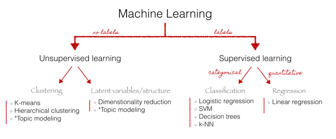
Source: Christine Doig 2015, also see Grimmer and Stewart (2013) for an overview of text as data methods.
7 Unsupervised: Topic Modeling (1)
- Goal: discovering the hidden (i.e, latent) topics within the documents and assigning each of the topics to the documents
- topic models belong to a class of unsupervised classification
- i.e., no prior knowledge of a corpus’ content or its inherent topics is needed (however some knowledge might help you validate your model later on)
- Researcher only needs to specify number of topics (not as intuitive as it sounds!)
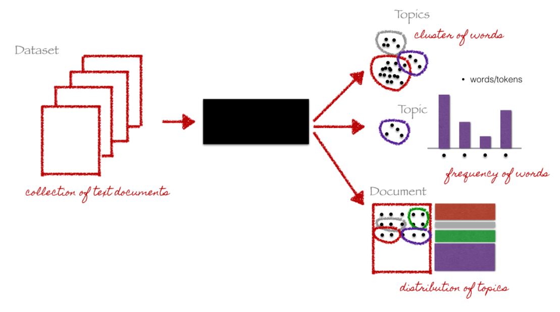
Source: Christine Doig 2015
8 Unsupervised: Topic Modeling (2)
- one of the most popular topic model algorithms
- developed by a team of computer linguists (David Blei, Andrew Ng und Michael Jordan, original paper)
- two assumptions:
- each document is a mixture over latent topics
- for example, in a two-topic model we could say “Document 1 is 90% topic A and 10% topic B, while Document 2 is 30% topic A and 70% topic B.”
- each topic is a mixture of words (with possible overlap)
- each document is a mixture over latent topics
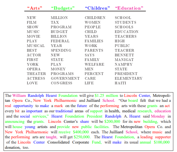
Note: Exemplary illustration of findings from an LDA on a corpus of news articles. Topics are mixtures of words. Documents are mixtures of topics. Source: Blei, Ng, Jordan (2003)
9 Preprocessing text
- Following chapter Tuning text models.
- Text must be heavily processed to be used as predictor data for modeling
- We pursue different steps:
- Create an initial set of count-based features, such as the number of words, spaces, lower- or uppercase characters, URLs, and so on; we can use the textfeatures package for this.
- Tokenize the text (i.e. break the text into smaller components such as words).
- Remove stop words such as “the”, “an”, “of”, etc.
- Stem tokens to a common root where possible.
- Remove predictors with a single distinct value.
- Center and scale all predictors.
- Important: More advanced preprocessing (transformers, BERT) is in the process of being implemented (see
textrecipes)- Right now still has to be done before (e.g., basic BERT with r)
10 Lab: Classifying text
Lab is based on an older lab by myself. The data comes from our project on measuring trust (see Landesvatter & Bauer (forthcoming) in Sociological Methods & Research). The data for the lab was pre-processed. 56 open-ended answers that revealed the respondent’s profession, age, area of living/rown or others’ specific names/categories, particular activities (e.g., town elections) or city were deleted for reasons of anonymity.
- Research questions: Do individuals interpret trust questions similar? Do they have a higher level if they think of someone personally known to them?
- Objective: Predict whether they think of personally known person (yes/no).
We start by loading our data that contains the following variables:
respondent_id: Individual’s identification number (there is only one response per individual - so it’s also the id for the response)social_trust_score: Individual’s value on the trust scale- Question: Generally speaking, would you say that most people can betrusted, or that you can’t be too careful in dealing with people? Please tell me on a score of 0 to 6, where 0 means you can’t be too careful and 6 means that most people can be trusted.
- Original scale: 0 - You can’t be too careful; 1; 2; 3; 4; 5; 6 - Most people can be trusted; Don’t know;
- Recoded scale:
Don't know = NAand values0-6standardized to0-1.
- Question: Generally speaking, would you say that most people can betrusted, or that you can’t be too careful in dealing with people? Please tell me on a score of 0 to 6, where 0 means you can’t be too careful and 6 means that most people can be trusted.
text: Individual’s response to the probing question- Question: In answering the previous question, who came to your mind when you were thinking about ‘most people?’ Please describe.
human_classified: Variable that contains the manual human classification of whether person was thinking about someone personally known to them or not (this is based on the open-ended response totext)N = 295were classified as1 = yesN = 666were classified as0 = noN = 482were not classified (we want to make predictions on those those!)
Table 1 shows the first few rows of the dataset:
| respondent_id | social_trust_score | text | human_classified |
|---|---|---|---|
| 1 | 0.5000000 | People I know or have known a while. | NA |
| 2 | 0.5000000 | Really everybody I know whether it be somebody I know as a neighbor or somebody I know as a friend somebody I know as a very close in a close relationship everybody has their limits of what they're capable of doing and they may hit a wall and get to a point where they I feel threatened and acted in the erratic way but most people if I'm treating them with gentleness and respect we will have a decent interaction. But I just never know depends on how things are shaping up what kind of day everybody's having. I suppose mostly I just have confidence in my ability to stay grounded in the flow of and Gestalt of interaction and find a current the river and float down the middle so to speak metaphorically. | 1 |
| 3 | 0.6666667 | I thought about people I've met recently. One is a woman I met at the dog park I've become friends with | 1 |
| 4 | 0.1666667 | Strangers and sometimes even work colleagues. | 1 |
| 5 | 0.3333333 | I was clearly thinking of coworkers, 2 in particular where trust depended on whether or not there was something to gain by them being trustworthy or not. What they could get away with to their benefit | 1 |
| 6 | 0.5000000 | Depends on the person. | NA |
The variable human_classified contains the values NA (was not classified), 1 (respondents were thinking about people known to them) and 0 (respondents were not thinking about people known to them).
10.1 Random Forest for text classification (with tuning)
- Steps
- Load and initial split of the data
- Create folds for cross-validation
- Define recipe (text preprocessing) & model (random forest + parameters to tune) & workflow
- 1st fitting & tuning session: Fit model to resampled training data (folds) + tuning in parallel and inspect accuracy & tuning parameters afterwards
- If happy,
select_besthyperparameters (identified in tuning),finalize_modelthe model with those parameters and create a finalworkflow_final. Train/fitworkflow_finalto the full training dataset and obtainfit_final. - Use
fit_finalto predict outcome both indata_trainanddata_testand evaluate accuracy. - To explore which predictors are important calcuculate and visualize variable importance.
We first import the data into R:
# Extract data with missing outcome
  data_missing_outcome <- data %>%
                  filter(is.na(human_classified))
  dim(data_missing_outcome)
[1] 482 4# Omit individuals with missing outcome from data
data <- data %>% drop_na(human_classified) # ?drop_na
dim(data)[1] 961 4# 1.
# Split the data into training and test data
set.seed(345)
data_split <- initial_split(data, prop = 0.8)
data_split # Inspect<Training/Testing/Total>
<768/193/961># Extract the two datasets
data_train <- training(data_split)
data_test <- testing(data_split) # Do not touch until the end!
# 2.
# Create resampled partitions of training data
data_folds <- vfold_cv(data_train, v = 2) # V-fold/k-fold cross-validation
data_folds # data_folds now contains several resamples of our training data # 2-fold cross-validation
# A tibble: 2 × 2
splits id
<list> <chr>
1 <split [384/384]> Fold1
2 <split [384/384]> Fold2# 3.
# Define the recipe & model
recipe1 <-
recipe(human_classified ~ respondent_id + text, data = data_train) %>%
update_role(respondent_id, new_role = "id") %>% # update role
step_tokenize(text) %>% # Tokenize text (split into words)
step_stopwords(text) %>% # Remove stopwords
step_stem(text) %>% # Text stemming
step_tokenfilter(text, max_tokens = 100) %>% # Filter max tokens
step_tf(text) # convert to term-feature matrix
# Extract and preview data + recipe (direclty with $)
data_preprocessed <- prep(recipe1, data_train)$template
dim(data_preprocessed)[1] 768 102tf_text_acquaint
0 1 2
746 21 1 # Specify model with tuning
model1 <- rand_forest(
mtry = tune(), # tune mtry parameter
trees = 1000, # grow 1000 trees
min_n = tune() # tune min_n parameter
) %>%
set_mode("classification") %>%
set_engine("ranger",
importance = "permutation") # potentially computational intensive
# Specify workflow (with tuning)
workflow1 <- workflow() %>%
add_recipe(recipe1) %>%
add_model(model1)
# 4. 1st fitting & tuning & evaluation of accuracy
# Specify to use parallel processing
doParallel::registerDoParallel()
set.seed(345)
tune_result <- tune_grid(
workflow1,
resamples = data_folds,
grid = 10 # choose 10 grid points automatically
)
tune_result# Tuning results
# 2-fold cross-validation
# A tibble: 2 × 4
splits id .metrics .notes
<list> <chr> <list> <list>
1 <split [384/384]> Fold1 <tibble [30 × 6]> <tibble [0 × 3]>
2 <split [384/384]> Fold2 <tibble [30 × 6]> <tibble [0 × 3]>tune_result %>%
collect_metrics() %>% # extract metrics
filter(.metric == "accuracy") %>% # keep accuracy only
select(mean, min_n, mtry) %>% # subset variables
pivot_longer(min_n:mtry, # convert to longer
values_to = "value",
names_to = "parameter"
) %>%
ggplot(aes(value, mean, color = parameter)) + # plot!
geom_point(show.legend = FALSE) +
facet_wrap(~parameter, scales = "free_x") +
labs(x = NULL, y = "accuracy")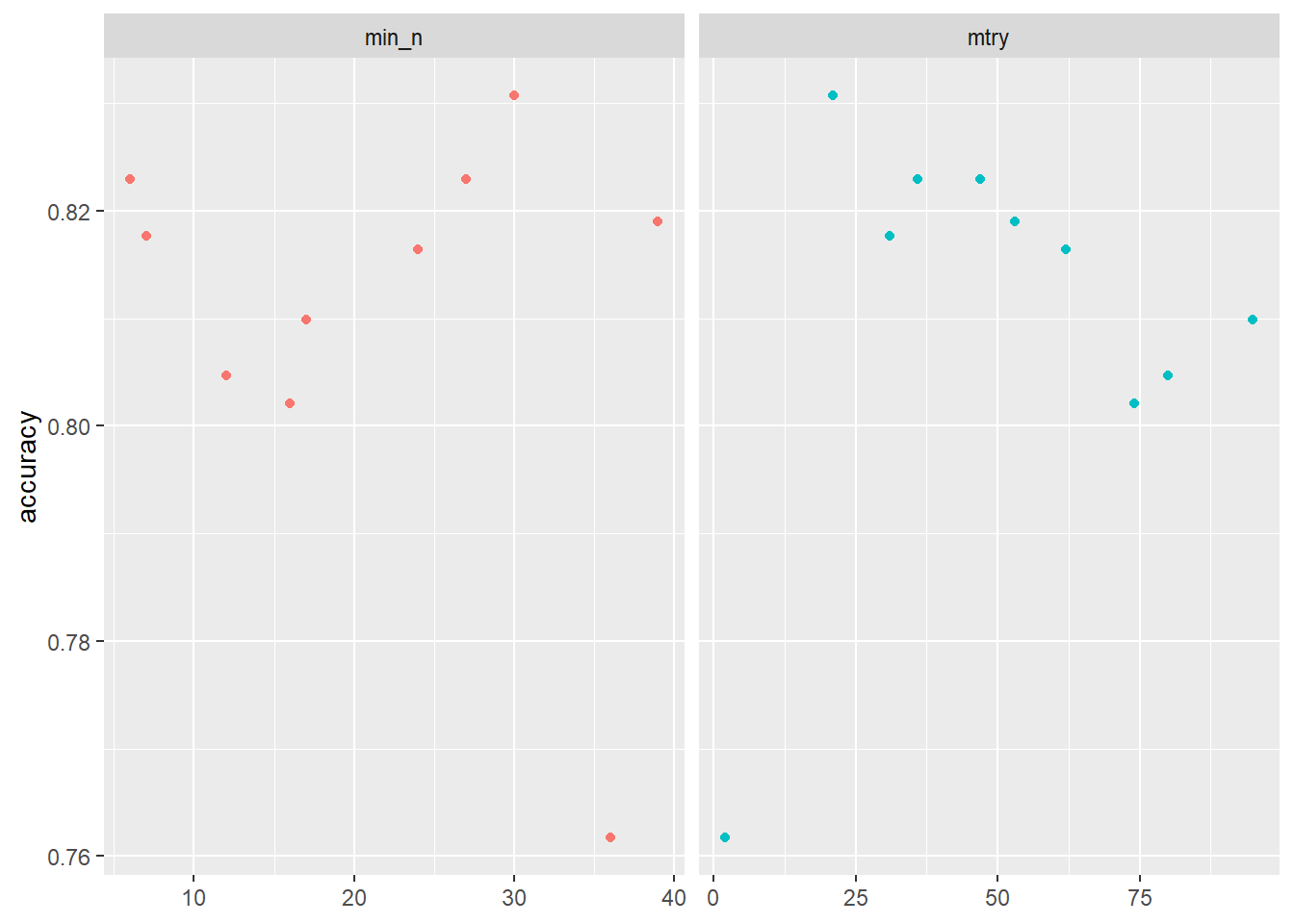
# 5. Choose best model after tuning & fit/train
  # Find tuning parameter combination with best performance values
  best_accuracy <- select_best(tune_result, metric = "accuracy")
  best_accuracy
# A tibble: 1 × 3
mtry min_n .config
<int> <int> <chr>
1 21 30 Preprocessor1_Model01 # Take list/tibble of tuning parameter values
# and update model1 with those values.
model_final <- finalize_model(model1, best_accuracy)
model_finalRandom Forest Model Specification (classification)
Main Arguments:
mtry = 21
trees = 1000
min_n = 30
Engine-Specific Arguments:
importance = permutation
Computational engine: ranger # Define final workflow
workflow_final <- workflow() %>%
add_recipe(recipe1) %>% # use standard recipe
add_model(model_final) # use final model
# Fit final model
fit_final <- parsnip::fit(workflow_final, data = data_train)
fit_final══ Workflow [trained] ══════════════════════════════════════════════════════════
Preprocessor: Recipe
Model: rand_forest()
── Preprocessor ────────────────────────────────────────────────────────────────
5 Recipe Steps
• step_tokenize()
• step_stopwords()
• step_stem()
• step_tokenfilter()
• step_tf()
── Model ───────────────────────────────────────────────────────────────────────
Ranger result
Call:
ranger::ranger(x = maybe_data_frame(x), y = y, mtry = min_cols(~21L, x), num.trees = ~1000, min.node.size = min_rows(~30L, x), importance = ~"permutation", num.threads = 1, verbose = FALSE, seed = sample.int(10^5, 1), probability = TRUE)
Type: Probability estimation
Number of trees: 1000
Sample size: 768
Number of independent variables: 100
Mtry: 21
Target node size: 30
Variable importance mode: permutation
Splitrule: gini
OOB prediction error (Brier s.): 0.1205772 # Q: What do the values for `mtry` and `min_n` in the final model mean?
# 6. Predict & evaluate accuracy (both in full training and test data)
metrics_combined <-
metric_set(accuracy, precision, recall, f_meas) # Set accuracy metrics
# Accuracy: Full training data
augment(fit_final, new_data = data_train) %>%
metrics_combined(truth = human_classified, estimate = .pred_class) # A tibble: 4 × 3
.metric .estimator .estimate
<chr> <chr> <dbl>
1 accuracy binary 0.895
2 precision binary 0.904
3 recall binary 0.947
4 f_meas binary 0.925# Cross-classification table
augment(fit_final, new_data = data_train) %>%
conf_mat(data = .,
truth = human_classified, estimate = .pred_class) Truth
Prediction 0 1
0 499 53
1 28 188# Accuracy: Test data
augment(fit_final, new_data = data_test) %>%
metrics_combined(truth = human_classified, estimate = .pred_class) # A tibble: 4 × 3
.metric .estimator .estimate
<chr> <chr> <dbl>
1 accuracy binary 0.860
2 precision binary 0.894
3 recall binary 0.914
4 f_meas binary 0.904# Cross-classification table
augment(fit_final, new_data = data_test) %>%
conf_mat(data = .,
truth = human_classified, estimate = .pred_class) Truth
Prediction 0 1
0 127 15
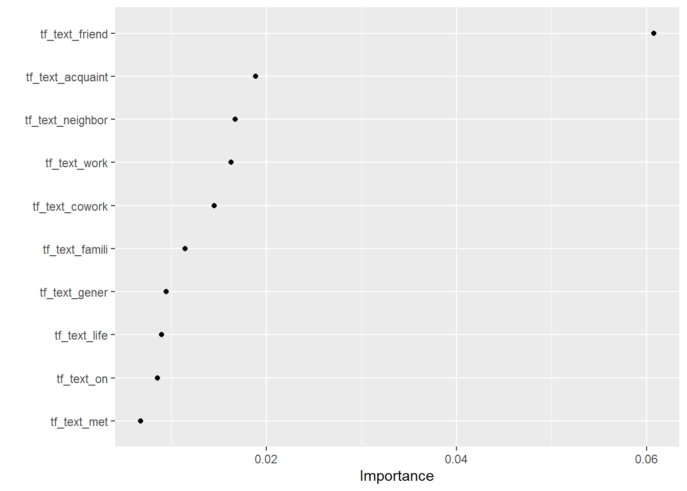
1 12 39# 7. Visualize variable importance
# install.packages("vip")
fit_final$fit$fit %>%
vip::vi() %>%
dplyr::slice(1:10) %>%
kable()| Variable | Importance |
|---|---|
| tf_text_friend | 0.0607590 |
| tf_text_acquaint | 0.0188360 |
| tf_text_neighbor | 0.0167197 |
| tf_text_work | 0.0162719 |
| tf_text_cowork | 0.0144992 |
| tf_text_famili | 0.0114177 |
| tf_text_gener | 0.0094499 |
| tf_text_life | 0.0089688 |
| tf_text_on | 0.0085111 |
| tf_text_met | 0.0067403 |
11 Exercise
- In the lab above we used a random forest to built a classifier for our labelled text. Thereby we made different choice in preprocessing the texts. Please modify those choices (e.g., don’t remove stopwords, change
max_tokens). How does this affect the accuracy of your model (and the training process)?
12 Lab: Classifying text using BERT
This lab was inspired by a lab by Dr. Hervé Teguim. The lab requires a working Python installation.
Below we install reticulate and the necessary python packages. We also import these packages/modules to make them available from within R in the virtual environment r-reticulate.
# Based on https://rpubs.com/Teguim/textclassificationwithBERT
# First set up the python environment to use: Global options -> Python


  library(reticulate) # To communicate with python

# List all available virtualenvs
  virtualenv_list()

# create a new environment
  virtualenv_create("r-reticulate")


# indicate that we want to use a specific virtualenv
  use_virtualenv("r-reticulate")

# install python packages
  virtualenv_install("r-reticulate", "pip")
  virtualenv_install("r-reticulate", "pandas")
  virtualenv_install("r-reticulate", "datasets")
  virtualenv_install("r-reticulate", "transformers")
  virtualenv_install("r-reticulate", "torch")
  virtualenv_install("r-reticulate", "scikit-learn")
  virtualenv_install("r-reticulate", "accelerate")


# Import python packages (so they are accessible in reticulate)
  pandas <- import("pandas")
  datasets <- import("datasets")
  transformers <- import("transformers")
  torch <- import("torch")
  accelerate <- import("accelerate")

# Change console from/to python: "reticulate::repl_python()" and with "exit"
We then import the data into R:
# Rename labelled data
  data <- data %>% rename(label = human_classified) %>%
  select(text, label) %>%
  mutate(label = as.numeric(as.character(label)))

# Extract data with missing outcome
  data_missing_outcome <- data %>%
                  filter(is.na(label))
  dim(data_missing_outcome)


# Omit individuals with missing outcome from data
  data <- data %>% drop_na(label) # ?drop_na
  dim(data)

# 1.
# Split the data into training, validation and test data
  set.seed(1234)
  data_split <- initial_validation_split(data, prop = c(0.6, 0.2))
  data_split # Inspect


# Extract the datasets
  data_train <- training(data_split)
  data_validation <- validation(data_split)
  data_test <- testing(data_split) # Do not touch until the end!
  dim(data_train)
Then we load the respective dataset into python so that we can access it there and save it in data.
# Load the dataset

#data = r.data_train # Get data from R into python
#len(data.index)

from datasets import DatasetDict

# Assuming you have your dataset 'train_dataset' ready


# Create a DatasetDict
data = DatasetDict()

data["train"] = r.data_train
data["train"]

data["validation"] = r.data_validation
data["validation"]

data["test"] = r.data_test
data["test"]


# We define a function dataframe_to_dataset(df) that takes a pandas DataFrame df as input and returns a Dataset object created from the DataFrame using Dataset.from_pandas(df).
# We iterate over the items in data.items(). For each key-value pair, we convert the value (pandas DataFrame) to a Dataset using the dataframe_to_dataset function, and assign the result back to the data DatasetDict at the same key.


# Conver
from datasets import Dataset, DatasetDict

# Assuming you have a DatasetDict named data with values train, validate, and test

# Function to convert pandas DataFrame to Dataset
def dataframe_to_dataset(df):
    return Dataset.from_pandas(df)

# Iterate over the items in the DatasetDict and convert pandas DataFrame to Dataset
for key, value in data.items():
    data[key] = dataframe_to_dataset(value)

# Now the values in the DatasetDict data are of type Dataset


data.map
exit
# CHANGE LABELS TO INTEGER
# TRAINING DATA
labels = data["train"]["label"] # Extract labels from the dataset
labels_int = [int(label) for label in labels] # Convert labels from float to int
data["train"] = data["train"].add_column("label_int", labels_int) # Update the dataset with the new integer labels
data["train"] = data["train"].remove_columns("label") # Optionally, you can remove the old float labels if you want to clean up the dataset
data["train"] = data["train"].rename_column("label_int", "label") # Rename the new 'label_int' column back to 'label'
print(data["train"]["label"][:5]) # Verify the changes
# VALIDATION DATA
labels = data["validation"]["label"] # Extract labels from the dataset
labels_int = [int(label) for label in labels] # Convert labels from float to int
data["validation"] = data["validation"].add_column("label_int", labels_int) # Update the dataset with the new integer labels
data["validation"] = data["validation"].remove_columns("label") # Optionally, you can remove the old float labels if you want to clean up the dataset
data["validation"] = data["validation"].rename_column("label_int", "label") # Rename the new 'label_int' column back to 'label'
print(data["validation"]["label"][:5]) # Verify the changes
# TEST DATA
labels = data["test"]["label"] # Extract labels from the dataset
labels_int = [int(label) for label in labels] # Convert labels from float to int
data["test"] = data["test"].add_column("label_int", labels_int) # Update the dataset with the new integer labels
data["test"] = data["test"].remove_columns("label") # Optionally, you can remove the old float labels if you want to clean up the dataset
data["test"] = data["test"].rename_column("label_int", "label") # Rename the new 'label_int' column back to 'label'
print(data["test"]["label"][:5]) # Verify the changes
data["train"]["label"]
data["validation"]["label"]
data["test"]["label"]This code segment imports the AutoTokenizer class from the transformers library and uses it to tokenize text data. It first defines the pre-trained model checkpoint name as “distilbert-base-cased” and initializes the tokenizer accordingly. Then, it defines a custom function called tokenize_function, which applies the tokenizer to each batch of text data, enabling padding and truncation. Finally, the function is applied to the data dataset, assuming it’s a dataset object with text data, using the map function with batched tokenization enabled for efficiency.
# Tokenization

# Import the AutoTokenizer class from the transformers module
from transformers import AutoTokenizer

# Define the pre-trained model checkpoint name
checkpoint = "distilbert-base-cased"

# Initialize the tokenizer using the pre-trained model checkpoint
tokenizer = AutoTokenizer.from_pretrained("distilbert-base-cased")

# Define a custom function to tokenize a batch of text data
def tokenize_function(batch):
    # Tokenize the text data in the batch, enabling padding and truncation
    return tokenizer(batch["text"], padding=True, truncation=True)

# Apply the tokenize_function to the data dataset, performing tokenization on each batch
# `data` is assumed to be a dataset object with text data to tokenize
# `batched=True` enables tokenization in batches for efficiency
# `batch_size=None` indicates that the dataset will be tokenized with the default batch size
data_encoded = data.map(tokenize_function, batched=True, batch_size=None)

# Show the sentence, the different tokens and the corresponding numerical ids
print(data_encoded['train'][0])

exit
Below a pre-trained model for sequence classification is defined using the Hugging Face Transformers library in Python. The AutoModelForSequenceClassification class is imported from the transformers module. The variable num_labels is assigned the number of output labels for the classification task, which is set to 2 here. The from_pretrained() method is then used to load a pre-trained DistilBERT model for sequence classification (‘distilbert-base-cased’). Additionally, the num_labels argument is specified to initialize the model with the correct number of output labels. This code initializes a model that is ready for training on a binary classification task.
# Definition of the model for training
from transformers import AutoModelForSequenceClassification

# Number of output labels for the classification task
num_labels = 2

# Load a pre-trained DistilBERT model for sequence classification and initialize it with the specified number of labels
# The 'distilbert-base-cased' checkpoint is used, which is a smaller version of the BERT model with cased vocabulary
model = AutoModelForSequenceClassification.from_pretrained('distilbert-base-cased',
                                                           num_labels=num_labels)

model

exit
We import the accuracy_score function from sklearn.metrics module to calculate the accuracy of predictions.
A function named get_accuracy is defined, which takes preds as input, representing the predictions made by a model.
Inside the function: * predictions variable is assigned the predicted labels obtained by taking the index of the maximum value along the last axis of the predictions tensor. This is done using the argmax() method. * labels variable is assigned the true labels extracted from the preds object. * The accuracy variable is assigned the accuracy score calculated by comparing the true labels and predicted labels using the accuracy_score function. * Finally, a dictionary containing the accuracy score is returned.
# Import the accuracy_score function from the sklearn.metrics module
from sklearn.metrics import accuracy_score

# Define a function to calculate the accuracy of predictions
def get_accuracy(preds):
    # Extract the predicted labels by taking the index of the maximum value along the last axis of the predictions tensor
    predictions = preds.predictions.argmax(axis=-1)
    # Extract the true labels from the preds object
    labels = preds.label_ids
    # Calculate the accuracy score by comparing the true labels and predicted labels
    accuracy = accuracy_score(preds.label_ids, preds.predictions.argmax(axis=-1))
    # Return a dictionary containing the accuracy score
return {'accuracy': accuracy}Below, we define various parameters for training our model using the Hugging Face Transformers library. We set parameters such as the batch size, number of training epochs, learning rate, weight decay, evaluation strategy, and logging settings. These parameters control how the model is trained, including how data is batched, how often training metrics are logged, and how evaluation is performed. These parameters play a crucial role in determining the performance and efficiency of the training process.
# Parameters for the model
# Importing the TrainingArguments class from the transformers module
from transformers import TrainingArguments

# Setting parameters for training
batch_size = 16  # Batch size for training
logging_steps = len(data_encoded["train"]) // batch_size  # Calculate the number of logging steps
model_name = "distilbert-base-cased-finetuned-data"  # Name for the fine-tuned model

# Creating an instance of TrainingArguments with specified parameters
training_args = TrainingArguments(
    output_dir=model_name,  # Output directory for model checkpoints and logs
    num_train_epochs=2,  # Number of training epochs
    learning_rate=2e-5,  # Learning rate for training
    per_device_train_batch_size=batch_size,  # Batch size per device for training
    per_device_eval_batch_size=batch_size,  # Batch size per device for evaluation
    weight_decay=0.01,  # Weight decay parameter for regularization
    evaluation_strategy="epoch",  # Evaluation strategy ("epoch" evaluates at the end of each epoch)
    disable_tqdm=False,  # Whether to disable tqdm progress bars during training
    logging_steps=logging_steps,  # Number of steps before logging training metrics
    log_level="error",  # Logging level for training
    optim='adamw_torch'  # Optimizer used for training (AdamW with PyTorch backend),

)


exit
This code segment trains a model using the Hugging Face Transformers library. It initializes a trainer object with the specified model, training arguments, dataset splits (training and validation), and tokenizer. The model is then trained using the train() method. After training, the trained model is saved using the save_model() method. Evaluation of the trained model on the validation dataset is performed using the evaluate() method to assess training and validation accuracy. Finally, predictions are generated on the test dataset data_encoded['test'] using the predict() method, and both predicted classes and true labels are extracted for further analysis.
# Model training

# Import the Trainer class from the transformers library
from transformers import Trainer

# Initialize the Trainer with the specified parameters
trainer = Trainer(model=model,  # Specify the model to be trained
                  args=training_args,  # Specify training arguments
                  compute_metrics=get_accuracy,  # Specify function to compute metrics
                  train_dataset=data_encoded["train"],  # Specify training dataset
                  eval_dataset=data_encoded["validation"],  # Specify validation dataset
                  tokenizer=tokenizer)  # Specify tokenizer

# Train the model
trainer.train()

## Save the model

# Save the trained model
trainer.save_model()

## Training and validation accuracy

# Evaluate the model on the validation dataset and print training and validation accuracy
trainer.evaluate()

## Get the predictions

# Get predictions on the test dataset
preds = trainer.predict(data_encoded['test'])

# Extract predicted classes
pred_class = preds.predictions.argmax(axis=-1)

# Extract true labels
label = preds.label_ids


exit
In this code snippet, a tibble dataframe named prediction is created, which contains two columns: pred_class representing the predicted classes (converted to factors), and label representing the true labels (also converted to factors). Subsequently, the metrics function is called, which computes various model evaluation metrics. In this instance, it computes the accuracy metric by comparing the predicted classes with the true labels from the prediction dataframe.
# Computing different model metrics

# Create a tibble dataframe containing predicted classes and labels, converting them to factors
prediction <- tibble(
  pred_class = as_factor(py$pred_class),
  label = as_factor(py$label)
)

# Compute accuracy metric using the `metrics` function, passing in the prediction dataframe along with the label and predicted class columns
# The `metrics` function calculates various metrics such as accuracy, precision, recall, etc.
# In this case, it computes accuracy by comparing the predicted classes with the true labels
metrics(prediction, label, pred_class)
In summary, this code calculates the confusion matrix using the true labels and predicted class labels from the prediction data frame, and then generates a heatmap visualization of the confusion matrix using ggplot2. This visualization helps to understand the performance of a classification model by showing how often each class is misclassified as another.
# Confusion matrix
# Calculate the confusion matrix using the conf_mat() function from the 'yardstick' package.
# This function takes two arguments: 'label' which represents the true labels and 'pred_class' which represents the predicted class labels.
# The '%>%' operator pipes the 'prediction' data frame into the conf_mat() function.
# Then, the resulting confusion matrix is piped into the autoplot() function from the 'ggplot2' package to visualize it as a heatmap.
prediction %>%
  conf_mat(label, pred_class) %>%
  autoplot(type = "heatmap")
In summary, this code snippet initializes a text classification pipeline using a pre-trained model specified by model_name. It then utilizes this pipeline to classify a sample text, 'This is not my idea of fun', and stores the result. The result would typically include the predicted label and the associated confidence score or probability, depending on the specific classifier used.
# Importing the required library
from transformers import pipeline

# Initializing a text classification pipeline with the specified model
# 'model_name' should be replaced with the name of the pre-trained model to be used
# This could be a model trained for text classification tasks like sentiment analysis,
# or any other similar task supported by the Hugging Face Transformers library
classifier = pipeline('text-classification', model=model_name)

# Using the initialized pipeline to classify a sample text
# The text provided as an argument ('This is not my idea of fun') will be passed to the classifier,
# which will assign it a label based on the model's predictions
result = classifier('This is not my idea of fun')
The code below classifier('This was beyond incredible') performs text classification using the classifier pipeline initialized earlier.
13 Labelling data: How to create a training dataset
First, we would load the full dataset that contains the texts. Below we have a dataset with tweets that we classify.
# Import data
  data <- read_csv("www/data/data_tweets_de.csv",
                   col_types = cols(.default = "c")) %>% # Make sure to read in columns as character (otherwise you will get problem with long numbers) %>%
    select(text) %>% # drop irrelevant variables
    mutate(text_id = row_number()) # Add unique identifier

# Store data with ID
  # Don't change data so that ID does not get lost
  write_excel_csv(data, "www/data/data_tweets_de_id.csv") # Store data with ID


# Load data
  set.seed(100) # set seed for random select
  data_for_coding <- read_csv("www/data/data_tweets_de_id.csv",
                 col_types = cols(.default = "c")) %>%
    sample_n(size = nrow(.)) %>% # Randomly reorder rows
    slice(1:1000) # Take the first 1000 observations as an example

# Why would we randomly reorder rows?
Then we store the data locally in an excel file. Make sure that any data you export or import always contains a unique classifier (we created one above called text_id). Use delim = ';#;' or something special as delimiter that is unique and does not appear in the text (excel seems to recognize a unique delimiter).
We open the excel file and save it under another name (to make sure it’s not overwritten again), e.g., data_for_coding_paul.csv if the person who codes the sample is called Paul.
In this new excel file we create a variable called human_classified (or any other name) and label as many observations as possible following our coding scheme.
Then we import the data file the contains the labeled outcome stored in human_classified.
And we can check how many we have classified (here I classified only few observations). And we would also merge the data with the original data.
   0    1 <NA>
17 11 972 After that we would basically proceed as described in the lab above. If you don’t want to export the full dataset for manual labeling chose a subset and join the datasets again later (just make sure you have a unique identifier for joining). Make sure to check whether the process is sound and does not overwrite anything.
Besides, it may make sense to label with several persons (intercoder reliability) and discuss tricky cases and code them together.
References
Grimmer, Justin, and Brandon M Stewart. 2013. “Text as Data: The Promise and Pitfalls of Automatic Content Analysis Methods for Political Texts.” Political Analysis: An Annual Publication of the Methodology Section of the American Political Science Association 21 (3): 267–97.
Silge, Julia, and David Robinson. 2017. Text Mining with R: A Tidy Approach. O’Reilly Media.
Wilkerson, John, and Andreu Casas. 2017. “Large-Scale Computerized Text Analysis in Political Science: Opportunities and Challenges.” Annual Review of Political Science 20 (1): 529–44.
Footnotes
Document-term matrix (DTM) is a mathematical representation of text data where rows correspond to documents in the corpus, and columns correspond to terms (words or phrases). DFM, also known as a document-feature matrix, is similar to a DTM but instead of representing the count of terms in each document, it represents the presence or absence of terms.↩︎