| \(\text{Unit i} \quad\) | \(Name \quad\) | \(X1_{i}^{Age} \quad\) | \(X2_{i}^{Educ.} \quad\) | \(D_{i}^{PublicCoverage} \quad\) | \(Y_{i}^{Lifesat.} \quad\) |
|---|---|---|---|---|---|
| 1 | Sofia | 29 | 1 | 1 | 3 |
| 2 | Sara | 30 | 2 | 1 | 2 |
| 3 | José | 28 | 0 | 0 | 5 |
| 4 | Yiwei | 27 | 2 | 1 | ? |
| 5 | Julia | 25 | 0 | 0 | 6 |
| 6 | Hans | 23 | 0 | 1 | ? |
| .. | .. | .. | .. | .. | .. |
| 1000 | Hugo | 23 | 1 | 0 | 8 |
Introduction
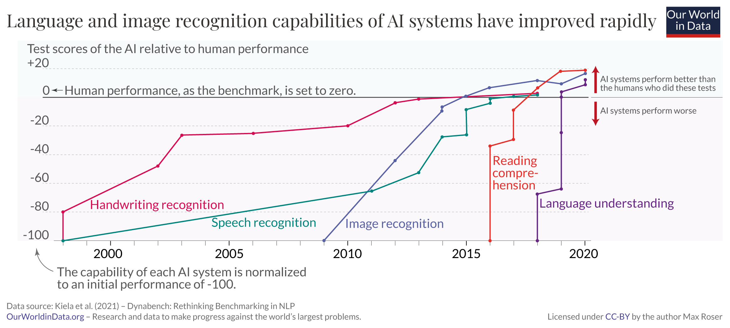
1 Capabilities of ML/AI models
2 Machine learning tasks in the social sciences
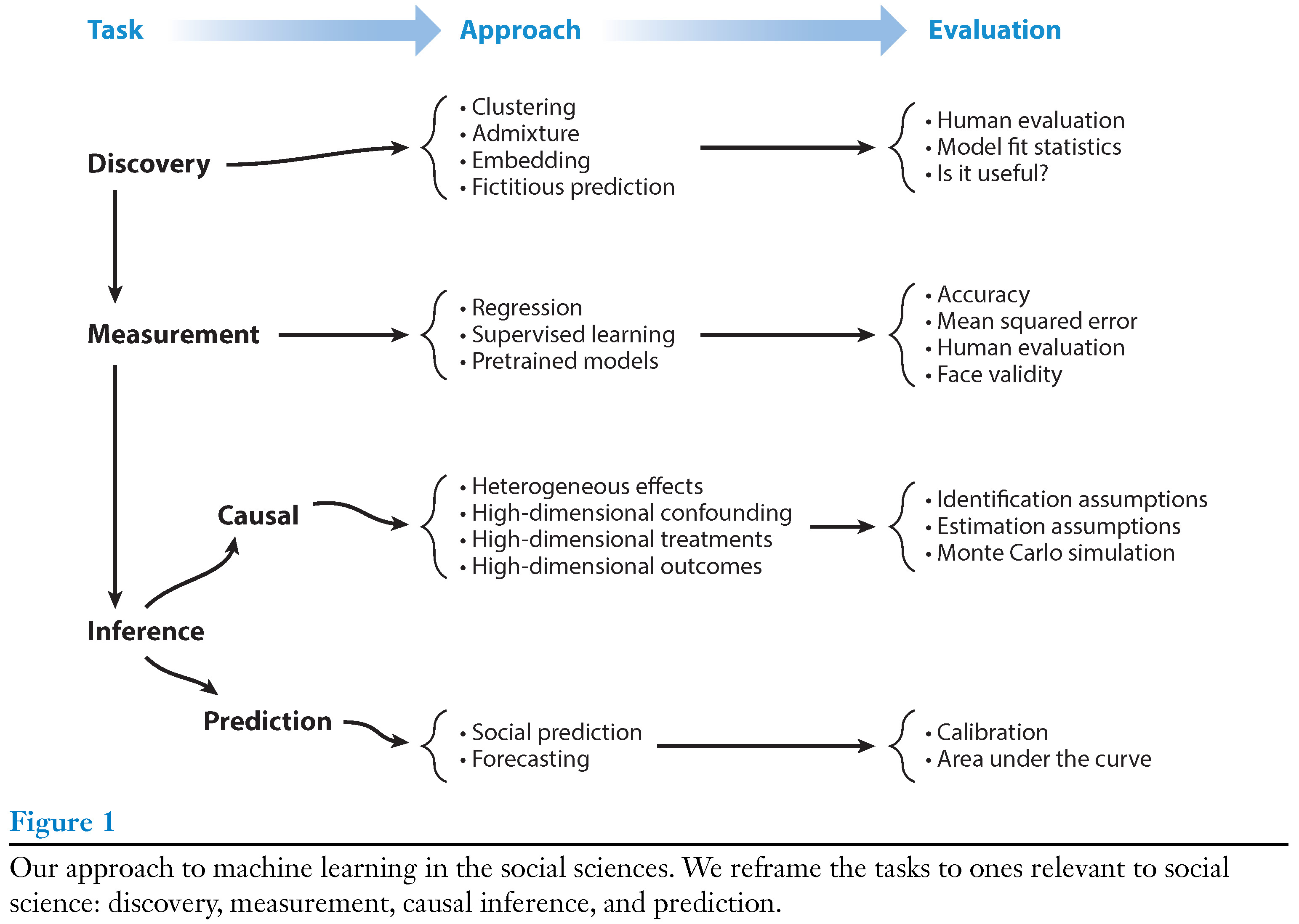
- Within social sciences ML is used for various tasks as summarized by Grimmer, Roberts, and Stewart (2021)1
- We’ll focus on prediction! (beware of ambiguity of “prediction”)
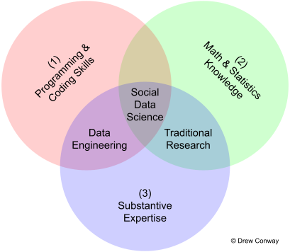
3 Predictive modelling: Skills
4 Terminology (1)
- Terminology is a source of confusion (Athey and Imbens 2019, 689)
- Q: Do you know any machine learning terminology?
- Statistical learning vs. machine learning (ML) (James et al. 2013, 1)
- Terms reflect disciplinary origin (statistics vs. computer science)
- We will use the two as synonyms (as well as AI)
- Regression problem: Prediction of a continuous or quantitative output values (James et al. 2013, 2)
- e.g., predict wage using age, education and year
- Classification problem: Prediction of a non-numerical value—that is, a categorical or qualitative output
- e.g., predict increase/decrease of stock market on a given day using previous movements
- Q: What does the “inference” in statistical inference stand for?^{Sample ← population.}
5 Terminology (2)
- Terminology: Well-established older labels vs. “new” terminology
- Sample used to estimate the parameters vs. training sample
- Model is estimated vs. Model is trained/fitted
- Independent variables, regressors, covariates, predictors vs. features (or inputs)
- Dependent variable/outcome vs. output/target
- Regression parameters (coefficients) vs. weights
6 Machine or statistical learning
7 Training, validation and test dataset
7.1 Training, validation and test dataset
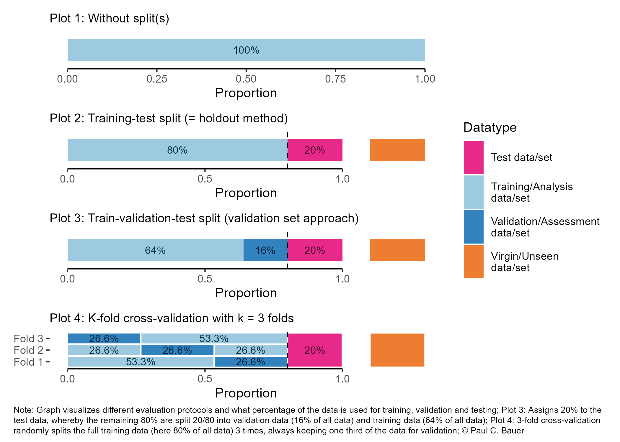
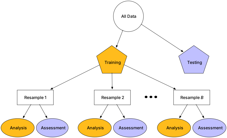
- As shown in Figure 1 when training models we sometimes…
- …only split into one training data subset, e.g., 80% of observations, and one test data subset, e.g., 20% of observations (cf. Plot 2)
- … introduce one further split (cf. Plot 3) - e.g., built models on training (analysis) dataset, validate/tune model using validation (assessment) dataset and use test dataset ONLY for final test
- …do resampling (see next slide!)
- As indicated in Figure 1, Plot 3 when doing further splitting the training data we can use the terms analysis and assessment dataset (Max Kuhn and Johnson 2019) (see also next slide)
7.2 Training, validation and test dataset: Resampling (several splits/folds)
- To avoid conceptual confusion we use the terminology by Max Kuhn and Johnson (2019) and illustrated in Figure Figure 2
- Datasets obtained from the initial split are called training and test data
- Datasets obtained from further splits to the training data are called analysis (analysis) and assessment (validation) datasets
- Often such further splits are called folds.
7.3 Training, validation and test dataset (3)
- Size of datasets: Usually 80/20 splits but depends..
- Q: What could be a problem if training and/or test dataset is too small? (uncertainty, representativeness)
Answer
- Training data ↓ → Variance of parameter estimates ↑
- Test data ↓ → Variance of performance statistic ↑
8 Assessing Model Accuracy
- See James et al. (2013, Ch. 4.4.3)
8.1 Assessing Model Accuracy: Classification
- Accuracy or Correct Classification Rate (CCR), i.e., the rate of correctly classified observations
- …the opposite of the error rate (e.g., James et al. 2013, chap. 2.2.3)
- Error rate: the proportion of mistakes that are made if we apply estimate to observations
- \(\frac{1}{n}\sum_{i=1}^{n}I(y_{i}\neq\hat{y}_{i})\): Fraction of incorrect classifications
- \(\hat{y}_{i}\): predicted class label for observation \(i\)
- \(I(y_{i}\neq\hat{y}_{i})\): indicator variable that equals 1 if \(y_{i}\neq\hat{y}_{i}\) (= error) and zero if \(y_{i}=\hat{y}_{i}\)
- If \(I(y_{i}\neq\hat{y}_{i})=0\) then the ith observation was classified correctly (otherwise missclassified)
- \(\frac{1}{n}\sum_{i=1}^{n}I(y_{i}\neq\hat{y}_{i})\): Fraction of incorrect classifications
- Training error rate vs. Test error rate
- Good classifier: One for which the test error rate is smallest
- Further measures2 later!
8.2 Assessing Model Accuracy: Error rate exercise
In Table 2 you find data (only 8 observations). Please assess/calculate the accuracy for those predictions for the dataset by calcuating the error rate.
- How do we proceed?
- Also, what role does the cutoff play?
- What role does the outcome distribution in the sample play?
| Name | public_coverage | public_coverage_num | prediction |
|---|---|---|---|
| Rie | No | 0 | 0.3 |
| Emily | Yes | 1 | 0.2 |
| Yohana | No | 0 | 0.5 |
| Stephanie | Yes | 1 | 0.2 |
| Sue | Yes | 1 | 0.8 |
| Cole | No | 0 | 0.2 |
| Madeeha | Yes | 1 | 1.0 |
| Hela | No | 0 | 0.1 |
Solution
- Below tables with the calculation steps for the error rate
- Get binary prediction. Usually cutoffs are \(p \geq 0.5 \rightarrow 1\) \(p<0.5 \rightarrow 0\), were \(p\) is the predicted probability.
- Get incorrect classifications/errors (1 = incorrect, 0 = correct) by comparing predicted (
prediction (binary)) with true values (public_coverage_num) - Sum up incorrect classifications & count observations
- Divide sum of incorrect classifications by number of observations
| Name | public_coverage_num | prediction | prediction (binary) | incorrect_classifications |
|---|---|---|---|---|
| Rie | 0 | 0.3 | 0 | 0 |
| Emily | 1 | 0.2 | 0 | 1 |
| Yohana | 0 | 0.5 | 1 | 1 |
| Stephanie | 1 | 0.2 | 0 | 1 |
| Sue | 1 | 0.8 | 1 | 0 |
| Cole | 0 | 0.2 | 0 | 0 |
| Madeeha | 1 | 1.0 | 1 | 0 |
| Hela | 0 | 0.1 | 0 | 0 |
| n | incorrect_classifications_sum | error_rate | ccr |
|---|---|---|---|
| 8 | 3 | 0.375 | 0.625 |
- Cutoff: The cutoff is the threshold that turns a probability score into a binary prediction. Here, the cutoff is 0.5: any prediction of 0.5 or higher is classified as ‘1’, and anything lower is classified as ‘0’. Changing this value alters the trade-off between correctly identifying positive cases (sensitivity) and correctly identifying negative cases (specificity).
- Outcome distribution: The outcome distribution in the sample refers to the proportion of each class (in this case, ‘Yes’ vs. ‘No’ or 1 vs. 0). Here, there are four 1s and four 0s, making it a perfectly balanced 50/50 distribution. This distribution is important because it provides a baseline for performance. In a balanced dataset, a model must perform better than 50% accuracy to be considered useful. If the sample were highly imbalanced (e.g., 90% ‘No’ and 10% ‘Yes’), a model could achieve 90% accuracy by simply predicting ‘No’ every time, making it seem effective when it’s actually not identifying any of the ‘Yes’ cases. Therefore, the distribution helps determine if accuracy is a meaningful metric for evaluation.
8.3 True/false negatives/positives
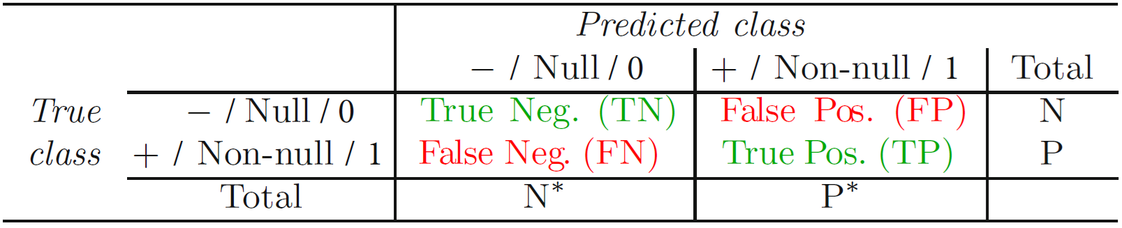
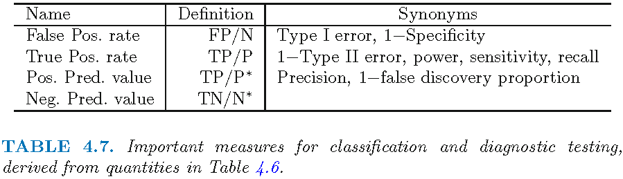
- Q: The tables in Figure 3 and Figure 4 illustrate how to calculate different accuracy metrics. Assuming the outcome is public coverage (1 = yes, 0 = no), how could we interpret the different cells?
8.4 Exercise: Accuracy measures
| 0 | 1 | ||
| 0 | 80 (TN) | 10 (FP) | 90 (N) |
| 1 | 5 (FN) | 5 (TP) | 10 (P) |
| 85 (N*) | 15 (P*) | 100 (total) |
8.5 Precision, recall & specificity
- Precision
- Focus: How many of the predicted 1s8 are true 1s?
- Interpretation: Precision is important when the cost of false positives is high, for example, in spam email detection, where you want to avoid marking a legitimate email as spam.
- Recall (Sensitivity)
- Focus: How many of the true 1s9 are predicted to be 1s?
- Interpretation: Recall is critical when missing a true positive has significant consequences, such as in medical diagnostics where you don’t want to miss a disease diagnosis.
- Specificity
- Focus: How many of the true 0s10 are predicted to be 0s?
- Interpretation: Specificity matters when it is crucial to correctly identify negative cases, such as in a test where false alarms are costly or burdensome, like unnecessary medical tests.
- …there are various other measures!
8.6 F1-score
- F1-Score as further popular measure
- \(F1 = 2 \times \frac{precision \times recall}{precision + recall} = \frac{2TP}{2TP+FP+FN}\)
- Highest possible value of an F-score is 1.0, indicating perfect precision and recall, and the lowest possible value is 0, if either precision or recall are zero
- F1-score combines both precision and recall into single score
- Precision measures accuracy of positive predictions; Recall measures how many actual positive instances were identified
- Useful when caring about both reducing false positives (high precision) and false negatives (high recall)
- Handles class imbalance better: considers both false positives and false negatives, providing a better sense of model’s performance with respect to the minority class
- Provides single metric for comparison
- BUT may mask underlying variation in precision/recall
8.7 Error rates and ROC curve
- Problem: Error rates are a function of the classification threshold
- If we lower the classification threshold (e.g., use a predicted probability of 0.3 as cutoff) we classify more items as positive (e.g. predict them to have public coverage reoffend), thus increasing both False Positives and True Positives (cf. James et al. 2013, Fig 4.7, p. 147)
- Goal: Knowing how error rates develop as a function of the classification threshold
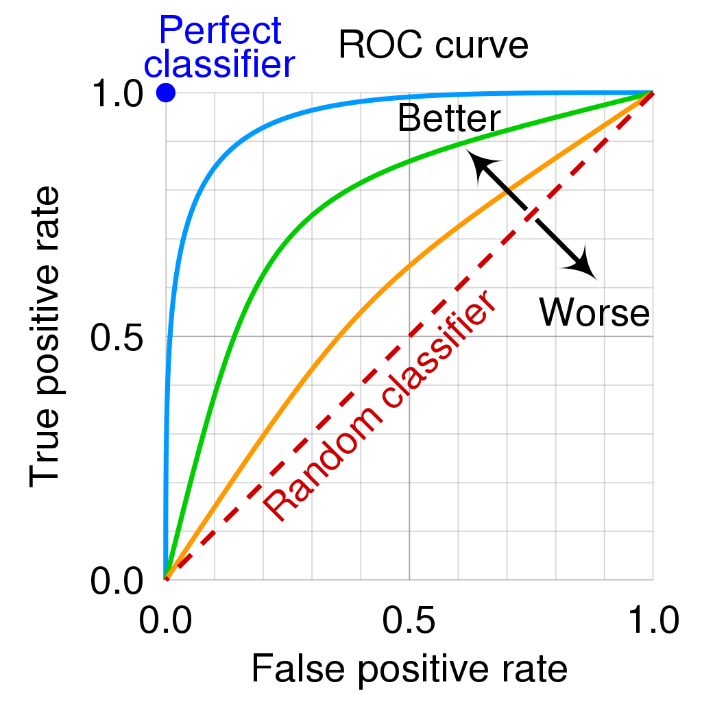
- Receiver Operating Characteristic (ROC) curve provides overall performance of a classifier11, summarized over all possible thresholds (James et al. 2013, 147)
- Area Under the Curve (AUC): values closer to 1 preferable (see Figure 5 → maximize TRP, minimize FPR!)
Mnemonic bridge (Eselsbrücke) for sensitivity & specificity
Imagine you’re using a metal detector to search for gold (positive instances/cases). A sensitive detector beeps at almost every piece of gold, so it detects many (high true positive rate).
Imagine the metal detector is supposed to find only gold and not react to other trash (like bottles or aluminum foil). A specific detector focuses on the gold and ignores the rest (low false positive rate).
- Sensitivity → Sniffer: Finds as many positives as possible, even if there are some false positives.
- Specificity → Selective: Focuses on correctly identifying negatives without false positives.
8.8 Example from Paul’s research
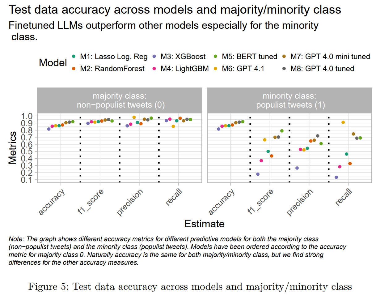
8.9 Weighting FPR and TPR differently (1)
Outcome: Public insurance coverage, where an individual is covered (1) or is not covered (0).
False Positive (FP): The model predicts an individual is covered by public insurance when they actually are not
- This could lead to administrative overhead and the misallocation of funds to ineligible individuals.
False Negative (FN): The model predicts an individual is not covered when they actually are.
- This is a critical error, as it could deny necessary healthcare access to an eligible person, potentially leading to severe health and financial consequences.
Assigning Costs:
- Cost of a False Positive (FP): Primarily administrative costs to correct the error. While not ideal, the impact is manageable.
- Cost of a False Negative (FN): Very high human and societal cost. An eligible person is left uninsured. This is probably more important to avoid.
8.10 Weighting FPR and TPR differently (2)
- Choosing a Threshold:
- Since the cost of a False Negative is much higher, our priority might be to minimize them.
- Minimizing the False Negative Rate (FNR) is equivalent to maximizing the True Positive Rate (TPR), because \(TPR = 1 - FNR\).
- Therefore, we should pick a threshold that yields a high TPR (correctly identifying as many covered individuals as possible), even if it means accepting a higher False Positive Rate (FPR).
- Important: The probability threshold used to classify someone as 0/1 is not directly visible on a standard ROC curve plot (like the one in Figure 5). It must be determined from the underlying data used to generate the curve.
8.11 Assessing Model Accuracy: Regression
- Mean squared error (James et al. 2013, Ch. 2.2)
- \(MSE=\frac{1}{n}\sum_{i=1}^{n}(y_{i}- \hat{f}(x_{i}))^{2}\) (James et al. 2013, Ch. 2.2.1)
- \(y_{i}\) is \(i\)s true outcome value
- \(\hat{f}(x_{i}) = \hat{y}_{i}\) is the prediction that \(\hat{f}\) gives for the \(i\)th observation
- MSE is small if predicted responses are to the true responses, and large if they differ substantially
- \(MSE=\frac{1}{n}\sum_{i=1}^{n}(y_{i}- \hat{f}(x_{i}))^{2}\) (James et al. 2013, Ch. 2.2.1)
- Training MSE: MSE computed using the training data
- Test MSE: How is the accuracy of the predictions that we obtain when we apply our method to previously unseen test data?
- Further measures
- Mean absolute error (MAE): …no squaring as in MSE
- R-squared: See Definitions -> Figure
- Fundamental property of ML (cf. James et al. 2013, 31, Figure 2.9)
- As model flexibility increases, training MSE will decrease, but the test MSE may not (danger of overfitting)
- Q: Why?
- As model flexibility increases, training MSE will decrease, but the test MSE may not (danger of overfitting)
More background
- Difference Between MSE, MAE, and R-squared in Prediction Accuracy: MSE is suitable for applications where larger errors need to be penalized more, MAE is preferable when the emphasis is on the overall accuracy without sensitivity to outliers, and R-squared is useful for assessing the overall goodness of fit of the model. However, it’s often recommended to use multiple metrics together to get a comprehensive understanding of model performance.
- Mean Squared Error (MSE):
- MSE calculates the average squared difference between the actual values and the predicted values.
- It emphasizes larger errors due to the squaring operation, making it sensitive to outliers.
- It is differentiable, making it useful for optimization algorithms.
- It penalizes large errors more than smaller ones, which may not always be desirable depending on the application.
- MSE can be heavily influenced by outliers, making it less robust in the presence of outliers.
- Mean Absolute Error (MAE):
- MAE calculates the average absolute difference between the actual values and the predicted values.
- It provides a more balanced view of errors compared to MSE as it is not as sensitive to outliers.
- It is more interpretable than MSE since it’s in the same units as the original data.
- It treats all errors equally regardless of their magnitude, which may not reflect the actual importance of errors in some cases.
- MAE is not differentiable at zero, which can complicate optimization tasks.
- R-squared (Coefficient of Determination):
- R-squared measures the proportion of the variance in the dependent variable that is predictable from the independent variables.
- It provides an indication of the goodness of fit of the model.
- R-squared ranges from 0 to 1, where 1 indicates perfect prediction and 0 indicates no improvement over a baseline model (usually the mean of the dependent variable).
- It is scale-independent, making it easier to compare models across different datasets.
- R-squared can be misleading when used alone, especially with complex models, as it can increase even when adding irrelevant predictors (overfitting).
- It assumes that the relationship between the dependent and independent variables is linear, which may not always be the case.
8.12 Assessing Model Accuracy: Exercise on MSE, MAE
| respondent_id | life_satisfaction | country | unemployed_active |
|---|---|---|---|
| 10608 | 5 | FR | 0 |
| 10405 | 8 | FR | 1 |
| 10007 | 7 | FR | 0 |
| 11170 | 10 | FR | 0 |
| 10751 | 10 | FR | 1 |
| 10005 | 10 | FR | 0 |
| .. | .. | .. | .. |
| Name | life_satisfaction | prediction (mean) | error |
|---|---|---|---|
| Arnela | 10 | 7.034 | 2.966 |
| Taryn | 7 | 7.034 | -0.034 |
| Thanaa | 7 | 7.034 | -0.034 |
| Blake | 5 | 7.034 | -2.034 |
| Chenell | 7 | 7.034 | -0.034 |
| Ryan | 10 | 7.034 | 2.966 |
| Dean | 8 | 7.034 | 0.966 |
| Edwin | 8 | 7.034 | 0.966 |
In Table 6 you find data (only 8 observations, i.e., a subset of the data above) and (like above) we use the mean as a predictive model. Please assess the accuracy for those predictions for the dataset by calcuating both the MSE and the MAE. How would we proceed? (Importantly, while we have only one dataset here and the mean model is based on this dataset, in ML applications the model is estimated based on some training data and the accuracy assessed with another datasetn namely validation or test data)
| Name | life_satisfaction | prediction (mean) | error |
|---|---|---|---|
| Arnela | 10 | 7.75 | 2.25 |
| Taryn | 7 | 7.75 | -0.75 |
| Thanaa | 7 | 7.75 | -0.75 |
| Blake | 5 | 7.75 | -2.75 |
| Chenell | 7 | 7.75 | -0.75 |
| Ryan | 10 | 7.75 | 2.25 |
| Dean | 8 | 7.75 | 0.25 |
| Edwin | 8 | 7.75 | 0.25 |
Solution
- Below tables with the calculation steps for the MSE
- Square the errors
- Sum up the squared errors & count observations
- Divide sum of squared errors by number of observations
| Name | life_satisfaction | prediction (mean) | error | error_squared |
|---|---|---|---|---|
| Arnela | 10 | 7.75 | 2.25 | 5.0625 |
| Taryn | 7 | 7.75 | -0.75 | 0.5625 |
| Thanaa | 7 | 7.75 | -0.75 | 0.5625 |
| Blake | 5 | 7.75 | -2.75 | 7.5625 |
| Chenell | 7 | 7.75 | -0.75 | 0.5625 |
| Ryan | 10 | 7.75 | 2.25 | 5.0625 |
| Dean | 8 | 7.75 | 0.25 | 0.0625 |
| Edwin | 8 | 7.75 | 0.25 | 0.0625 |
| n | error_squared_sum | MSE |
|---|---|---|
| 8 | 19.5 | 2.4375 |
- Below tables with the calculation steps for the MAE
- Get absolute values of errors
- Sum up the absolute values of errors & count observations
- Divide sum of absolute values of errors by number of observation
| Name | life_satisfaction | prediction (mean) | error | error_absolute |
|---|---|---|---|---|
| Arnela | 10 | 7.75 | 2.25 | 2.25 |
| Taryn | 7 | 7.75 | -0.75 | 0.75 |
| Thanaa | 7 | 7.75 | -0.75 | 0.75 |
| Blake | 5 | 7.75 | -2.75 | 2.75 |
| Chenell | 7 | 7.75 | -0.75 | 0.75 |
| Ryan | 10 | 7.75 | 2.25 | 2.25 |
| Dean | 8 | 7.75 | 0.25 | 0.25 |
| Edwin | 8 | 7.75 | 0.25 | 0.25 |
| n | error_absolute_sum | MSA |
|---|---|---|
| 8 | 10 | 1.25 |
9 Universal workflow of machine learning
- Source: Adapted from Chollet and Allaire (2018, 118f)
- Define the problem at hand and the data on which you’ll be training. Collect this data, or annotate it with labels if need be.
- Choose how you’ll measure success on your problem. Which metrics will you monitor on your validation data?
- Determine your evaluation protocol: hold-out validation? K-fold validation? Which portion of the data should you use for validation?
- Preparing/preprocess your data
- Develop a first model that does better than a basic baseline: a model with statistical power.
- Develop a model that overfits.
- Regularize your model and tune its hyperparameters, based on performance on the validation data.
- Final training (on all training + validation data) and model testing on unseen test dataset
Often Step 5, 6, and 7 are subsumed under one step Training & validation.
10 Software in R: Tidymodels & packages
- See github website.
10.1 Overview of packages
- A collection of packages for modeling and machine learning using tidyverse principles (see Barter (2020), M. Kuhn and Wickham (2020) and M. Kuhn and Silge (2022) for summaries)
- Much like
tidyverse,tidymodelsconsists of various core packages:rsample: for sample splitting (e.g. train/test or cross-validation)- provides functions to create different types of resamples and corresponding classes for their analysis
initial_split: Use this to split the data into training and test data (with argumentsprop,strata)prop-argument: Specify share of training data observationsstrata-argument: Conduct stratified sampling on the dependent variable (better if classes are imbalanced!)training(),testing(),analysis()andassessment()can be used to extract the corresponding datasets from anrsplitobjectvalidation_split: Split the training data into analysis data (= training data) and assessment data (= validation data)- Later we’ll explore more functions such as
vfold_cv
- Later we’ll explore more functions such as
recipes: for pre-processing- Use dplyr-like pipeable sequences of feature engineering steps to get your data ready for modeling.
parsnip: specifying the model namely model type, engine and mode- Goal: provide a tidy, unified interface to access models from different packages
model type-argument: e.g, linear or logistic regressionengine-argument: R packages that contain these modelsmode-argument: either regression or classification
tune: for model tuning- Goal: facilitate hyperparameter tuning. It relies heavily on
recipes,parsnip, anddialsdials: contains infrastructure to create and manage values of tuning parameters
- Goal: facilitate hyperparameter tuning. It relies heavily on
yardstick: evaluate model accuracy- Goal: estimate how well models are working using tidy data principles
conf_mat(): calculates cross-tabulation of observed and predicted classesmetrics(): estimates 1+ performance metrics
workflowsets:- Goal: allow users to create and easily fit a large number of different models.
- Use
workflowsetsto create aworkflow setthat holds multipleworkflow objects- These objects can be created by crossing all combinations of preprocessors (e.g., formula, recipe, etc) and model specifications. This set can be tuned or resampled using a set of specific functions.
10.2 ML workflow using tidymodels
| Data resampling, feature engeneering | Model fitting, tuning | Model evaluation |
|---|---|---|
| rsample | tune | yardstick |
| recipes | parsnip | |
| dials |
11 Appendix: Prediction models (general form)
11.1 Prediction: Model (general form)
- cf. James et al. (2013, 16–21)
- Output variable \(Y\), e.g., life satistfaction, trust, unemployment, recidivism
- Often called the response/dependent variable
- Input variable(s) \(X\) (usually with subscript, e.g., \(X_{1}\) is education)
- Usually called predictors/independent variables/features
- Example
- Quantitative response \(Y\) and \(p\) different predictors, \(X_{1},...,X_{p}\)
- We assume a relationship between output \(Y\) and inputs \(X = X_{1},...,X_{p}\)
- can be written generally as \(Y = f(X) + \varepsilon\)
- \(f\) represents the systematic information that \(X\) provides about \(Y\)
- \(\varepsilon\) is a random error term which is independent of \(X\) and has mean zero
- \(f\) is “true” function/model that produced \(Y\), e.g., the “true” function/model that produces life satisfaction given the inputs
- can be written generally as \(Y = f(X) + \varepsilon\)
11.2 Prediction: Why estimate \(f\) (model)?
Pertains to class distinction discussed in (Breiman 2001; James et al. 2013, 17–19)
Prediction: In many situations, a set of inputs \(X\) readily available, but true output values \(Y\) cannot be easily obtained, e.g., 20% of persons in a survey did not indicate their life satisfaction
- In this setting, since the error term averages to zero, we can predict true values \(Y\) using \(\hat{Y} = \hat{f}(X)\)
- where \(\hat{f}\) represents our estimate for \(f\), and \(\hat{Y}\) represents the resulting prediction for \(Y\)
- \(f\) is “true” function that produced \(Y\), e.g., “true” function/model that produces life satisfaction
- \(f\) is often treated as a black box, i.e., typically we are less concerned with exact form of \(\hat{f}\) provided that the predictions are accurate
- In this setting, since the error term averages to zero, we can predict true values \(Y\) using \(\hat{Y} = \hat{f}(X)\)
Inference: Understand the relationship between \(Y\) and \(X\)14
11.3 Prediction: Accuracy
- Accuracy of \(\hat{Y}\) as prediction for \(Y\) depends on two quantities
- reducible error (introduced by innaccuracy of \(\hat{f}\)) and the irreducible error (associated with \(\varepsilon\))
- \(\hat{f}\) will not be a perfect estimate of \(f\) but introduce error
- This error is reducible because we can potentially improve the accuracy of \(\hat{f}\) by using the most appropriate statistical learning technique to estimate \(f\)
- But even with perfect estimate of \(f\) (estimate response with form \(\hat{Y} = f (X)\)) error remains because \(Y\) is also function of \(\varepsilon\) that cannot be predicted using \(X\)
- Variability associated with \(\varepsilon\) also affects predictions and is called irreducible error
- Q: Why is the irreducible error (always) larger than 0?
Answer
The quantity \(\varepsilon\) may contain unmeasured variables that are useful in predicting \(Y\): since we don’t measure them, \(f\) cannot use them for its prediction. The quantity may also contain unmeasurable variation (James et al. 2013, 18–19).
Irreducible error will always provide an upper bound on the accuracy of our prediction for Y. This bound is almost always unknown in practice since we may not have measured/know the necessary features/predictors. (James et al. 2013, 19)
11.4 Prediction: How Do We Estimate f?
We estimate \(f\) using the training data (James et al. 2013, 21–24)
Parametric methods with two-step approach (James et al. 2013, 21–24)
- Make assumption about the functional form of \(f\), or shape, e.g., linear model
- Train or fit the model, e.g., most common method for linear model is (ordinary) least squares
- “parametric” because assumpions about data distribution (e.g., linear) and reduces problem of estimating \(f\) down to estimating a set of parameters, e.g., coefficients of linear model
- Potential disadvantage
- the model we choose will usually not match the true unknown form of \(f\)
- if too far from true \(f\) then estimate will be poor
- Flexible models can fit many different function forms for \(f\) but require estimating more parameters but increase danger of overfitting (Q: Overfitting?)
Non-parametric methods (e.g. random forests)
- Do not make explicit assumptions about the functional form of \(f\)
- Seek estimate of \(f\) that gets as close to the data points as possible without being too rough or wiggly
11.5 Trade-Off(s): Prediction Accuracy vs. Model Interpretability
- Some ML methods are more some are less flexible (shape of f), e.g., linear model
- James et al. (2013, 25), Fig. 2.7. provides an overview
- Q: Why would we ever choose to use a more restrictive method (less flexible) model instead of a very flexible approach?
Answer
- Inference: If main goal is inference, restrictive models are much more interpretable. Linear model may be a good choice since it will be quite easy to understand the relationship between \(Y\) and \(X_{1}, ..., X_{p}\)
- Prediction
- High flexibility can also yield worse predictions because of overfitting (counterintuitive!)
- Debate around interpretable machine learning: Sometime we would like to know why a model predicts well (which features matter how much!)
- See Molnar (2022)
12 Appendix: Bias/variance trade-off and accuracy
Learning outcomes/objective: Learn/understand…
- …bias-variance trade-off.
12.1 Bias-variance trade-off
- See James et al. (2013, Ch. 2.2.2)
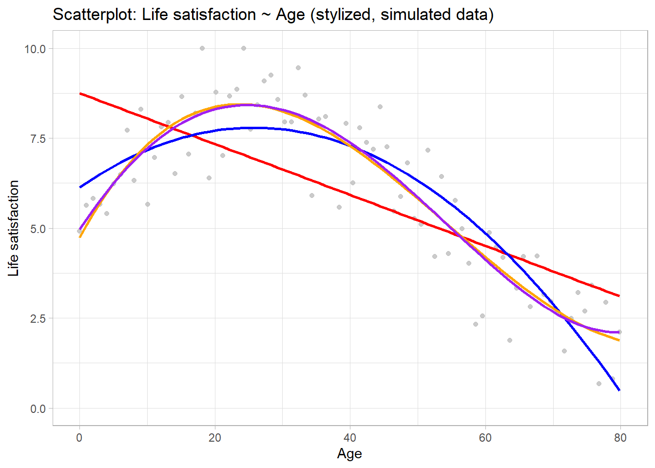
- Figure 8 shows an increasingly flexible model (linear model + polynomials)
12.1.1 Bias-variance trade-off (1)
- James et al. (2013) introduce bias-variance trade-off before turning to classification
- What do we mean by the variance and bias of a statistical learning method? (James et al. 2013, Ch. 2.2.2)
- Variance refers to amount by which \(\hat{f}\) would change if estimated using a different training data set
- Ideally estimate for \(f\) should not vary too much between training sets
- If method has high variance then small changes in training data can result in large changes in \(\hat{f}\)
- More flexible methods/models usually have higher variance
- Bias refers to the error that is introduced by approximating a (potentially complicated) real-life problem through a much simpler model (=\(f\))
- e.g., linear regression assumes linear relationship between \(Y\) and \(X_{1},X_{2},...,X_{p}\) but unlikely that real-life problems truly have linear relationship producing bias/error
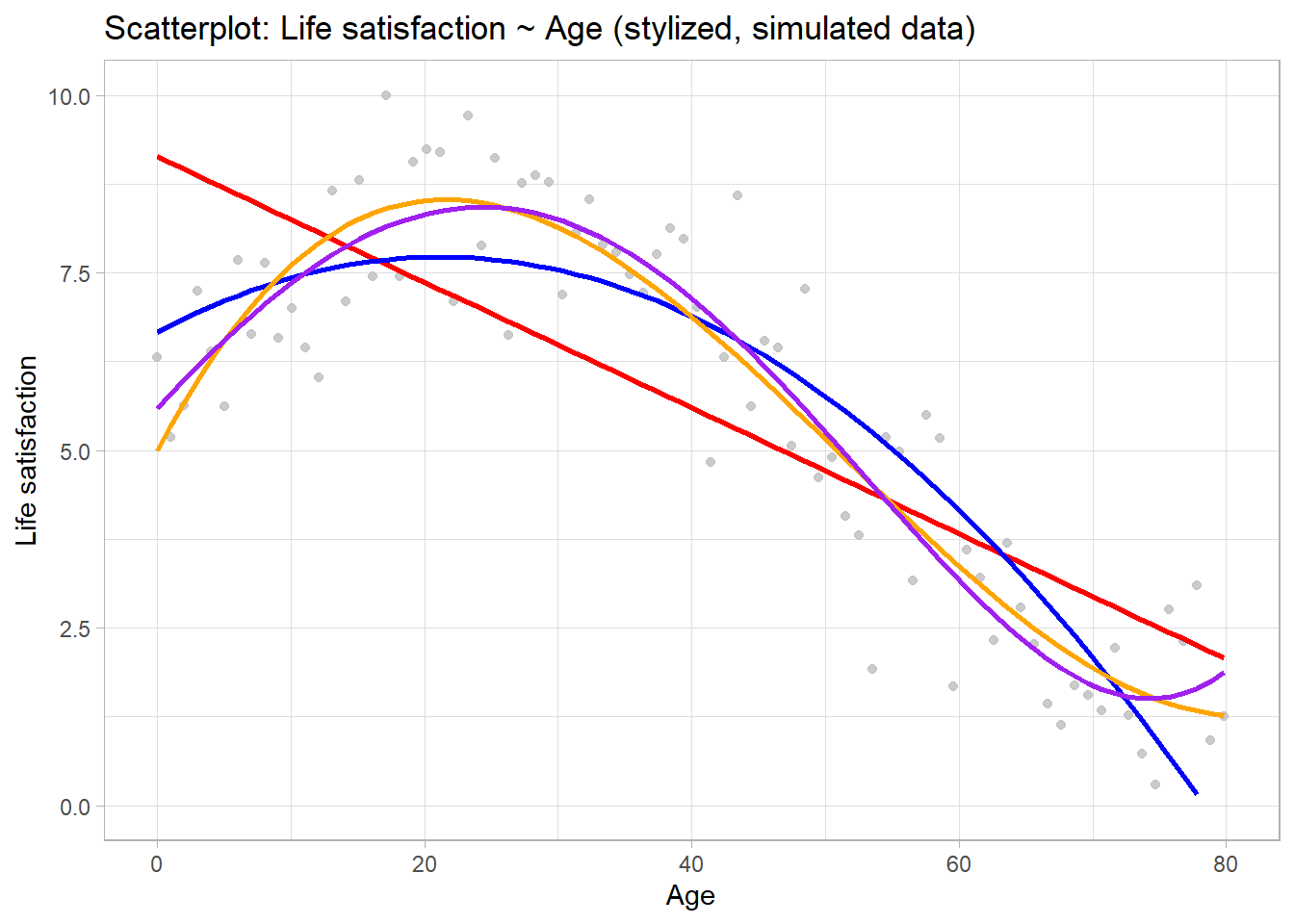
- e.g., predict life satisfaction \(Y\) with age \(X\)
- If real-life \(f\) is substantially non-linear, linear regression will not produce accurate estimate \(\hat{f}\) of \(f\), no matter how many training observations
- Variance refers to amount by which \(\hat{f}\) would change if estimated using a different training data set
12.1.2 Bias-variance trade-off (2)
- Variance: error from sensitivity to small fluctuations in the training set
- High variance may result from an algorithm modeling the random noise in the training data (overfitting)
- Bias error: error from erroneous assumptions in the learning algorithm (\(\hat{f}\)) about \(f\)
- High bias can cause an algorithm to miss relevant relations between features and target outputs (underfitting)
- Bias-variance trade-off: Property of model that variance of parameter(s) estimated across samples can be reduced by increasing the bias in the estimated parameters
- e.g., we may choose linear model with higher bias to decreas variance
- Bias-variance dilemma/problem: Trying to simultaneously minimize these two sources of error that prevent supervised learning algorithms from generalizing beyond their training set
12.1.3 Bias-variance trade-off (3)
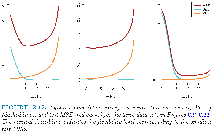
- “General rule”: with more flexible methods/models, variance will increase and bias will decrease
- Relative rate of change of these two quantities determines whether test MSE (regression problem) increases or decreases
- As we increase flexibility of a class of methods, bias tends to initially decrease faster than the variance increases
- Consequently, the expected test MSE declines as shown in Figure 9.
- Q: What does Figure 9 illustrate and which level of flexibility would be desirable?
Answer
- Figure 9 visualizes squared bias, variance and MSE as a function of flexibility. We would normally pick a flexibility level that minimizes all three of them (indicated by the vertical dashed line).
12.1.4 Bias-variance trade-off (4)
- Good test set performance requires low variance as well as low squared bias
- Trade-off because easy to obtain method with…
- …extremely low bias but high variance
- e.g., just draw a curve that passes through every single training observation
- …very low variance but high bias
- e.g., by fitting a horizontal line to the data
- …extremely low bias but high variance
- Trade-off because easy to obtain method with…
- Challenge lies in finding a method for which both the variance and the squared bias are low
- In real-life situation \(f\) is unobserved hence not possible to compute test MSE, bias, or variance for a statistical learning method (because we fit our model to the training data not the test data!)
- But good to keep in mind and later on we discuss methods to estimate test MSE using training (cross-validation!)
12.2 Exercise 1
Adapted from James et al. (2013, Exercise 2.4.1): Thinking of our classification problem (predicting recidivism, i.e., whether a prisoner reoffends), indicate whether we would generally expect the performance of a flexible statistical learning method to be better or worse than an inflexible method. Justify your answer.
- The sample size \(n\) is extremely large, and the number of predictors \(p\) is small.
- The number of predictors \(p\) is extremely large, and the number of observations \(n\) is small.
- The relationship between the predictors and response is highly non-linear.
- The variance of the error terms, i.e. \(\sigma^{2}=Var(\epsilon)\), is extremely high.
Answer
- Flexible is better since there is less room for adaption to outliers!
- Flexible is worse since function will adapt non-typical outliers!
- Flexible is better because the function should adapt the non-linear true function f.
- Flexible is probably better because it would better adapt to the high variance, i.e., high variance seems to indicate that non-flexible model is not a good approximation of f.
12.3 Exercise 2
James et al. (2013, Exercise 2.4.2): Explain whether each scenario is a classification or regression problem, and indicate whether we are most interested in inference or prediction. Finally, provide \(n\) and \(p\).
- We collect a set of data on the top 500 firms in the US. For each firm we record profit, number of employees, industry and the CEO salary. We are interested in understanding which factors affect CEO salary.
- We are considering launching a new product and wish to know whether it will be a success or a failure. We collect data on 20 similar products that were previously launched. For each product we have recorded whether it was a success or failure, price charged for the product, marketing budget, competition price, and ten other variables.
- We are interesting in predicting the % change in the US dollar in relation to the weekly changes in the world stock markets. Hence we collect weekly data for all of 2012. For each week we record the % change in the dollar, the % change in the US market, the % change in the British market, and the % change in the German market.
Answer
- Regression problem; Inference; n = 500; p = 3 (profit, number of employees, industry)
- Classification problem; Prediction; n = 20; p = 14 (success or failure, price charged for the product, marketing budget, competition price, and ten other variables)
- Regression problem; Prediction; n = 52; p = 4; (% change in the dollar, the % change in the US market, the % change in the British market, and the % change in the German market)
13 Appendix: Regression vs. Classification
Variables can be characterized as either quantitative or qualitative (= categorical)
Quantitative variables: Numerical values, e.g., person’s age, height, or income,
Qualitative variables: Values in one of K different classes, or categories
- e.g., a person’s gender (male or female)
Q: Are the following variables quantitative (A) or qualitative (B)?
- brand of product purchased, (2) wether a person defaults on a debt, (3) value of a house, (4) cancer diagnosis (Acute Myelogenous Leukemia, AcuteLymphoblastic Leukemia, or No Leukemia), (5) price of a stock
Problems with quantitative response = regression problems
Problems with qualitative response = classification problems
Distinction is not always crisp, e.g., logistic regression
- Typically used with a qualitative (two-class, or binary) response
- But estimates are class probabilities
Source: James et al. (2013, chap. 2.1.5)
13.1 Exercise: Classification or regression?
Classification problems occur often, perhaps even more so than regression problems, e.g., :
- A person arrives at the emergency room with a set of symptoms that could possibly be attributed to one of three medical conditions. Which of the three conditions does the individual have?
- An online banking service must be able to determine whether or nota transaction being performed on the site is fraudulent, on the basis of the user’s IP address, past transaction history, and so forth.
- On the basis of DNA sequence data for a number of patients with and without a given disease, a biologist would like to figure out which DNA mutations are deleterious (disease-causing) and which are not.
If we have a set of training observations (\(x_{1},y_{1}\)),…,(\(x_{n},y_{n}\)), we can build a classifier
Why not linear regression?
- No natural way to convert qualitative response variable with more than two levels into a quantitative response for LM
- e.g., 1 = stroke, 2 = drug overdose, 3 = epileptic seizure
- and linear probability model for binary outcome provides predictions outside of [0,1] interval (James et al. 2013, 131, Figure 4.2)
- No natural way to convert qualitative response variable with more than two levels into a quantitative response for LM
Source: James et al. (2013, chaps. 4.1, 4.2)
13.2 Classification: Two-class (binary) vs. multi-class problems
- Many classification involve several classes…
- …but can usually be reframed as (multiple) two-class
- e.g., Religion: Predicting whether someone is protestant vs. all others
- Logistic regression restricted to two-class problems by default
- Other models allow for predicting several classes (e.g., multinomial logistic regression)
References
Athey, Susan, and Guido W Imbens. 2019. “Machine Learning Methods That Economists Should Know About.” Annu. Rev. Econom. 11 (1): 685–725.
Barter, Rebecca. 2020. “Tidymodels: Tidy Machine Learning in R.” https://www.rebeccabarter.com/blog/2020-03-25_machine_learning/#what-is-tidymodels.
Breiman, Leo. 2001. “Statistical Modeling: The Two Cultures (with Comments and a Rejoinder by the Author).” SSO Schweiz. Monatsschr. Zahnheilkd. 16 (3): 199–231.
Chollet, Francois, and J J Allaire. 2018. Deep Learning with R. 1st ed. Manning Publications.
Grimmer, Justin, Margaret E Roberts, and Brandon M Stewart. 2021. “Machine Learning for Social Science: An Agnostic Approach.” Annu. Rev. Polit. Sci. 24 (1): 395–419.
James, Gareth, Daniela Witten, Trevor Hastie, and Robert Tibshirani. 2013. An Introduction to Statistical Learning: With Applications in R. Springer Texts in Statistics. Springer.
Kuhn, Max, and Kjell Johnson. 2019. Feature Engineering and Selection: A Practical Approach for Predictive Models. CRC press (Taylor & Francis).
Kuhn, M, and J Silge. 2022. “Tidy Modeling with R.”
Kuhn, M, and H Wickham. 2020. “Tidymodels: A Collection of Packages for Modeling and Machine Learning Using Tidyverse Principles.” Boston, MA, USA.
Molnar, Christoph. 2022. “Interpretable Machine Learning.” https://christophm.github.io/interpretable-ml-book/.
Salganik, Matthew J, Ian Lundberg, Alexander T Kindel, Caitlin E Ahearn, Khaled Al-Ghoneim, Abdullah Almaatouq, Drew M Altschul, et al. 2020. “Measuring the Predictability of Life Outcomes with a Scientific Mass Collaboration.” Proc. Natl. Acad. Sci. U. S. A. 117 (15): 8398–8403.
Footnotes
Clustering: a technique for grouping units into inductively determined, mutually exclusive, and exhaustive sets; Admixture: similar to cluster analysis but representing each unit with a set of proportions (nonnegative weights that sum to one) that represent membership across all clusters; Embedding: mapping of units to a low-dimensional, real-valued vector that contains information about the unit; Fictitious prediction problem: a prediction problem where the goal is to learn the features that enable prediction; the predictions themselves are not of interest↩︎
e.g., precision, recall (sensitivity), F1 score, ROC AUC↩︎
The No Information Rate (NIR) is the accuracy that could be achieved by always predicting the most frequent class in the dataset. If in a dataset 70% of the samples belong to class A (public_coverage = yes = 1), the NIR would be 70%, since predicting class A for every sample would result in 70% accuracy.↩︎
# of true positive (TP) divided by # of actually positive individuals (P = TP + FN). Example: # of individuals that have public coverage AND are predicted to have public coverage (true positives TP) – divided by – # of individuals that have public coverage (P)↩︎
# of true positive (TP) divided by # of predicted positive individuals (P*= TP + FP), including those not identified correctly. Example: # of individuals that have public coverage AND are predicted to have public coverage (true positives TP) – divided by – # of individuals predicted to have public coverage (P*)↩︎
# of true negative (TN) divided by # of actually negative individuals (N = TN + FP). Example: # of individuals that don’t have public coverage AND are predicted to NOT have public coverage (true negatives TN) – divided by – # of all individuals that don’t have public coverage (N)↩︎
Accuracy = 85%; Sensitivity = 50%; Specificity = 88.89%; Precision = 33.33%↩︎
Those predicted to have have public coverage.↩︎
Those who have public coverage.↩︎
Those who don’t have public coverage.↩︎
False positive rate (FPR): \(FP/N\) \(=\) \(1 - specificity\); True positives rate (TPR): \(TP/P\) \(=\) \(sensitivity\) (James et al. 2013, Fig 4.8, p. 148)↩︎
The probability threshold used to classify someone as 0/1 is not directly visible on a standard ROC curve plot. It must be determined from the underlying data used to generate the curve.↩︎
Share of populist tweets in test data is around 14%.↩︎
See corresponding questions in James et al. (2013, 19–20)↩︎