Outlook: Further interpretability methods

1 Ceteris Paribus Plots

1.1 Overview

• Ceteris Paribus (CP) Plots: Show a single feature’s effect on one prediction.
• Latin for “other things equal”.
• Isolate one feature’s impact while keeping all others constant.
• The fundamental building block for other methods:
  • ICE Plot: A collection of all CP curves for a dataset.
  • PDP: The average of all CP curves in a dataset.
• See algorithm in Molnar (2022)
• For code see chapter in Biecek and Burzykowski (2021)

1.2 CP Plots: Strengths and Limitations

• Strengths
  • Simple to implement and understand¹
  • Complement attribution methods (SHAP/LIME)²
  • Flexible building blocks³
• Limitations
  • Only shows one feature change at a time⁴
  • Interpretation suffers with correlated features⁵
  • High risk of wrongful causal interpretation⁶

1.3 Lab R

1.3.1 Prepare data and train model

First, we’ll run your setup code to train our Random Forest model on the public_coverage data.

library(knitr)
library(tidymodels)
library(dplyr)
library(readr)
library(DALEX)
library(ceterisParibus) # Load the ceterisParibus package

# Load and prepare data
#data <- read_csv(url(sprintf("https://docs.google.com/uc?id=%s&export=download",
#                         "1dnCK79T45Qa7RZrDg1qv6-EdGBoxCPjv")))
data <- read_csv("data/data_acspubliccoverage.csv")
data <- data %>% mutate(across(where(is.character), as.factor))

# Split the data
set.seed(123)
data_split <- initial_split(data, prop = 0.80, strata = public_coverage)
data_train <- training(data_split)
data_test  <- testing(data_split)

# Define the recipe and model spec
recipe_rf <- recipe(public_coverage ~ ., data = data_train) %>%
  step_impute_median(all_numeric_predictors()) %>% # Impute numeric NAs
  step_impute_mode(all_nominal_predictors())      # Impute categorical NAs
model_rf <- rand_forest(mode = "classification") %>% set_engine("ranger")

# Create and fit the workflow
workflow_rf <- workflow() %>%
  add_recipe(recipe_rf) %>%
  add_model(model_rf)
fit_rf <- fit(workflow_rf, data = data_train)

1.3.2 Create a DALEX Explainer

The ceterisParibus package is part of the DALEX ecosystem, so it needs a DALEX explainer object to work with our model. We will create an explainer that focuses on predicting the probability of the “Yes” class for public_coverage.

# Define the predict function for the "Yes" class probability
p_fun <- function(object, newdata) {
  predict(object, new_data = newdata, type = "prob")$.pred_Yes
}

# Create the explainer for our tidymodels workflow
explainer <- explain(
  model = fit_rf,
  data = select(data_test, -public_coverage),
  y = data_test$public_coverage == "Yes",
  predict_function = p_fun,
  label = "Random Forest",
  type = "classification",
  verbose = FALSE
)

1.3.3 Create and Plot Ceteris Paribus Profiles

Now, we select an individual from our test set and create Ceteris Paribus plots for him/her. The plot will show how the model’s prediction for that person would change if we varied his/her feature values one at a time, keeping all other features constant. * Below Top observations describes the data of the original, unchanged person we asked the model to explain. * Top profiles: contain the Ceteris Paribus simulation that shows what the model would have predicted (yhat) for this same person if only their income had been different, while all other features (age, education, etc.) were held constant.

observation_to_explain <- select(data_test, -public_coverage) %>% slice(1)

cp_data_rf <- predict_profile(explainer = explainer, 
                           new_observation = observation_to_explain)


cp_data_rf

Top profiles    : 
  income age          education marital_status    sex         disability
1      0  23 High School or GED  Never married Female Without disability
2    300  23 High School or GED  Never married Female Without disability
3    600  23 High School or GED  Never married Female Without disability
4    900  23 High School or GED  Never married Female Without disability
5   1200  23 High School or GED  Never married Female Without disability
6   1500  23 High School or GED  Never married Female Without disability
  parent_employment           citizenship   mobility military_service ancestry
1              <NA> Citizen by birth (US) Same house     Never served   Single
2              <NA> Citizen by birth (US) Same house     Never served   Single
3              <NA> Citizen by birth (US) Same house     Never served   Single
4              <NA> Citizen by birth (US) Same house     Never served   Single
5              <NA> Citizen by birth (US) Same house     Never served   Single
6              <NA> Citizen by birth (US) Same house     Never served   Single
  nativity hearing_difficulty vision_difficulty cognitive_difficulty
1   Native                 No                No                   No
2   Native                 No                No                   No
3   Native                 No                No                   No
4   Native                 No                No                   No
5   Native                 No                No                   No
6   Native                 No                No                   No
         employment gave_birth            race    _yhat_ _vname_ _ids_
1 Employed Civilian         No Some Other Race 0.2987949  income     1
2 Employed Civilian         No Some Other Race 0.2366688  income     1
3 Employed Civilian         No Some Other Race 0.2580072  income     1
4 Employed Civilian         No Some Other Race 0.2740474  income     1
5 Employed Civilian         No Some Other Race 0.2967339  income     1
6 Employed Civilian         No Some Other Race 0.2777668  income     1
        _label_
1 Random Forest
2 Random Forest
3 Random Forest
4 Random Forest
5 Random Forest
6 Random Forest


Top observations:
  income age          education marital_status    sex         disability
1   5000  23 High School or GED  Never married Female Without disability
  parent_employment           citizenship   mobility military_service ancestry
1              <NA> Citizen by birth (US) Same house     Never served   Single
  nativity hearing_difficulty vision_difficulty cognitive_difficulty
1   Native                 No                No                   No
         employment gave_birth            race    _yhat_       _label_ _ids_
1 Employed Civilian         No Some Other Race 0.2666677 Random Forest     1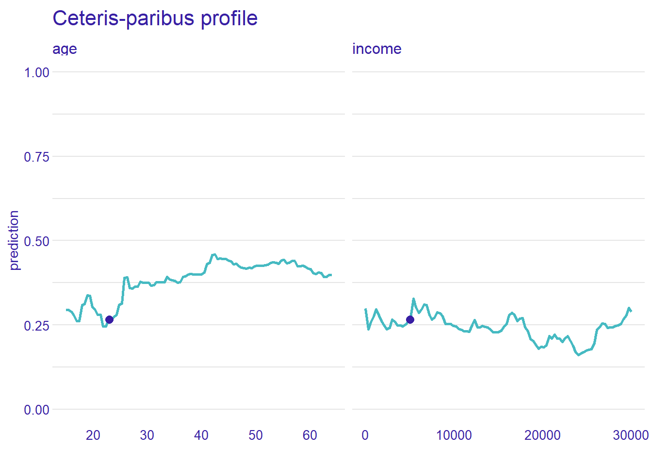

plot(cp_data_rf, variables = c("age", "income")) +
  ggtitle("Ceteris-paribus profile", "") + ylim(0, 1)

Ceteris Paribus profiles for 5 individuals, colored by sex.

This plot contains a panel for each continuous variable (like age and income).

• Within each panel:
  • The x-axis shows the range of possible values for that feature.
  • The y-axis shows the model’s predicted probability of having public coverage.
  • The plot shows what the model would have predicted for that person if only that one feature had been different.

2 Counterfactual Explanations

2.1 Introduction: The “What If” Explanation

• LIME: “Why did the model decide this?”
• Counterfactual: “What could I do to change the decision?”
• Specific “what if” scenarios to flip outcomes (e.g., “loan denied” \(\rightarrow\) “loan approved”).
• Analogy: GPS shows the wrong location.
  • LIME (Why): “You are here because you turned left on Main St.”
  • Counterfactual (How): “To get there, go back and turn right on Main St.”
• Focus on actionable advice \(\rightarrow\) A cornerstone of responsible AI.

Source: https://github.com/interpretml/DiCE

2.2 How Counterfactuals are Generated

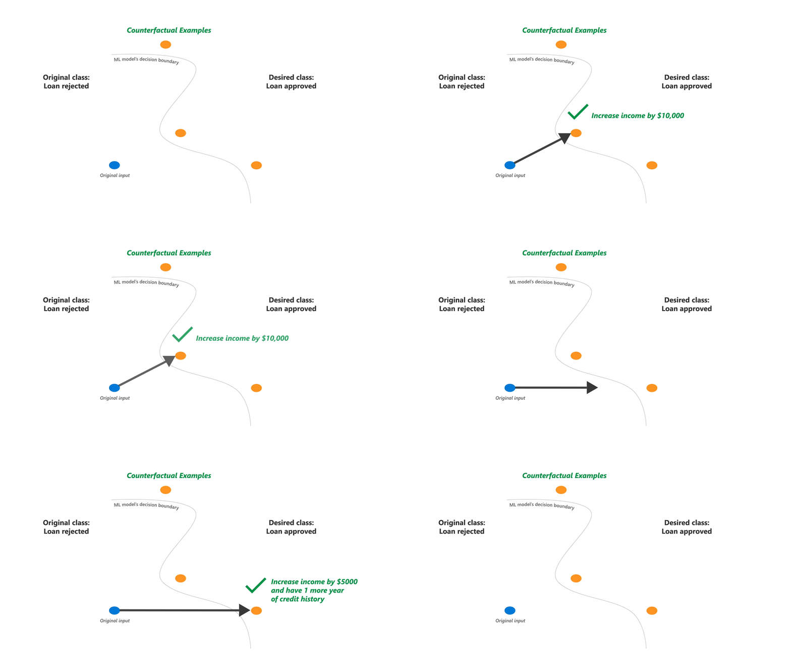
• Goal: Smallest data change for the desired prediction.
• Core Idea: Algorithm finds a nearby, hypothetical point that “flips” the outcome.
• Process: An optimization problem with two goals:
  1. New point gets the desired prediction.
  2. Changes from the original point are minimal.

2.3 Key Properties of Good Counterfactuals

• Sparsity: Minimal feature changes (e.g., “increase income by $5k” vs. 10 changes).
• Actionability: Changes must be possible (e.g., no immutable features like age).
• Plausibility: The resulting hypothetical data point must be realistic.

2.4 Counterfactuals and Fairness

• A direct way to implement fairness via actionable recourse.
• Providing Recourse: A clear path to appeal or change automated decisions (fulfills legal needs, e.g., GDPR).
• Uncovering Bias: The counterfactuals themselves can reveal deep model biases.
  • Unequal Burdens: Man told “increase salary by $5k,” woman told “$15k” for the same outcome.
  • Unrealistic Suggestions: Consistently less plausible paths for one group \(\rightarrow\) model bias.

2.5 Summary & Key Takeaways

• “What if” explanations that provide actionable advice.
• Answers: “What must change for a better outcome?”
• Found by seeking the smallest feature change that flips the prediction.
• A key fairness tool: provides recourse and audits if the “path to success” is fair for all groups.

2.6 Lab R

In this exercise, we will use the counterfactuals package to answer the question: “For a person predicted to not have public coverage, what are the smallest changes to their features that would flip the prediction to Yes?”

In this exercise, we will use the counterfactuals package to find out what would need to change for an individual to receive a different prediction from our model. We’ll train a randomForest model and then find counterfactuals for a person who the model predicts does not have public health coverage. * Problem: We can not simply use the tidymodels pipeline because counterfactuals does not know how to properly interpret tidymodels objects. We tidymodels to prepare our data but then resort to the simple randomForest function.

library(counterfactuals)
library(randomForest)
library(iml)
library(tidymodels)
library(dplyr)
library(readr)
library(tidyr) # For handling NAs

2.6.1 1. Fitting a model

First, we load and prepare our data. The randomForest function cannot handle missing values, so we will remove any rows with NAs from our training data for this exercise. To do so we recur to functions prep and bake from the tidymodels workflow. Then, we train the model to predict public_coverage.

# Load and prepare data
data <- read_csv("data/data_acspubliccoverage.csv")
data <- data %>% mutate(across(where(is.character), as.factor))

# Split the data
set.seed(123)
data_split <- initial_split(data, prop = 0.80, strata = public_coverage)
data_train <- training(data_split)
data_test  <- testing(data_split)



# Define the recipe and model spec
  recipe_rf <- recipe(public_coverage ~ ., data = data_train) %>%
    step_impute_median(all_numeric_predictors()) %>%
    step_impute_mode(all_nominal_predictors())
  prepped_recipe <- prep(recipe_rf, data_train)
  baked_train_data <- bake(prepped_recipe, new_data = data_train)

# Train the model on the complete training data
rf_model <- randomForest(public_coverage ~ ., data = baked_train_data)

2.6.2 2. Setting up an iml::Predictor Object

Next, we create an iml::Predictor object. This is a wrapper that contains our trained model and the data used to train it, which the counterfactuals package needs to work.

predictor <- Predictor$new(
  rf_model, 
  data = select(data_train_complete, -public_coverage), 
  y = data_train_complete$public_coverage,
  type = "prob"
)

2.6.3 3. Finding Counterfactuals

Now, let’s find an interesting person from our test set to explain. We’ll pick someone for whom the model predicts they do not have public coverage and find out what would need to change for them to be predicted as “Yes”.

# Find a person in the test set predicted as "No" with high confidence
# We must use a complete case for the explanation
person_of_interest <- data_test %>%
  drop_na() %>%
  filter(predict(rf_model, newdata = .) == "No") %>%
  slice(1)
person_of_interest

# A tibble: 1 × 19
  public_coverage income   age education     marital_status sex    disability   
  <fct>            <dbl> <dbl> <fct>         <fct>          <fct>  <fct>        
1 No                   0    17 No HS Diploma Never married  Female Without disa…
# ℹ 12 more variables: parent_employment <fct>, citizenship <fct>,
#   mobility <fct>, military_service <fct>, ancestry <fct>, nativity <fct>,
#   hearing_difficulty <fct>, vision_difficulty <fct>,
#   cognitive_difficulty <fct>, employment <fct>, gave_birth <fct>, race <fct>

# Check the model's original prediction for this person
# The model is very sure this person's class is "No"
original_prediction <- predictor$predict(person_of_interest)
original_prediction

     No   Yes
1 0.792 0.208

# We want to find changes that would make the 
# prediction for class "Yes" at least 50%
whatif_classif <- WhatIfClassif$new(predictor, n_counterfactuals = 5L)

# Find the counterfactuals
cfactuals <- whatif_classif$find_counterfactuals(
  person_of_interest, 
  desired_class = "Yes", 
  desired_prob = c(0.5, 1)
)

2.6.4 4. The Counterfactuals Object

The cfactuals object contains the results. We can now print it to see a summary, view the data, and plot the findings to understand the suggested changes.

First, let’s see the summary of the counterfactuals found.

cfactuals

5 Counterfactual(s) 
 
Desired class: Yes 
Desired predicted probability range: [0.5, 1] 
 
Head: 
   income   age     education marital_status    sex         disability
    <num> <num>        <fctr>         <fctr> <fctr>             <fctr>
1:      0    17 No HS Diploma  Never married Female Without disability
2:      0    17 No HS Diploma  Never married Female Without disability
3:      0    17 No HS Diploma  Never married Female Without disability
         parent_employment           citizenship   mobility military_service
                    <fctr>                <fctr>     <fctr>           <fctr>
1:    2 parents, both work Citizen by birth (US) Same house     Never served
2: 2 parents, mother works Citizen by birth (US) Same house     Never served
3:    Mother only, no work Citizen by birth (US) Same house     Never served
       ancestry nativity hearing_difficulty vision_difficulty
         <fctr>   <fctr>             <fctr>            <fctr>
1: Not reported   Native                 No                No
2:       Single   Native                 No                No
3:       Single   Native                 No                No
   cognitive_difficulty         employment gave_birth                      race
                 <fctr>             <fctr>     <fctr>                    <fctr>
1:                   No Not in labor force         No           Some Other Race
2:                   No Not in labor force         No Black or African American
3:                   No Not in labor force         No                     White

The counterfactuals are stored in the .data field of the cfactuals object. Each row is a slightly modified version of our original person that now gets the desired prediction.

kable(cfactuals$data)

income	age	education	marital_status	sex	disability	parent_employment	citizenship	mobility	military_service	ancestry	nativity	hearing_difficulty	vision_difficulty	cognitive_difficulty	employment	gave_birth	race
0	17	No HS Diploma	Never married	Female	Without disability	2 parents, both work	Citizen by birth (US)	Same house	Never served	Not reported	Native	No	No	No	Not in labor force	No	Some Other Race
0	17	No HS Diploma	Never married	Female	Without disability	2 parents, mother works	Citizen by birth (US)	Same house	Never served	Single	Native	No	No	No	Not in labor force	No	Black or African American
0	17	No HS Diploma	Never married	Female	Without disability	Mother only, no work	Citizen by birth (US)	Same house	Never served	Single	Native	No	No	No	Not in labor force	No	White
0	17	No HS Diploma	Never married	Female	Without disability	Mother only, works	Citizen by birth (US)	Same house	Never served	Multiple	Native	No	No	No	Not in labor force	No	White
0	17	High School or GED	Never married	Female	Without disability	Mother only, works	Citizen by birth (US)	Same house	Never served	Not reported	Native	No	No	No	Not in labor force	No	White

With the evaluate() method, we can see how good our counterfactuals are. Lower is generally better for dist_x_interest (less change) and no_changed (fewer features changed).

kable(cfactuals$evaluate())

income	age	education	marital_status	sex	disability	parent_employment	citizenship	mobility	military_service	ancestry	nativity	hearing_difficulty	vision_difficulty	cognitive_difficulty	employment	gave_birth	race	dist_x_interest	no_changed	dist_train	dist_target	minimality
0	17	No HS Diploma	Never married	Female	Without disability	2 parents, both work	Citizen by birth (US)	Same house	Never served	Not reported	Native	No	No	No	Not in labor force	No	Some Other Race	0.0555556	1	0	0	0
0	17	No HS Diploma	Never married	Female	Without disability	2 parents, mother works	Citizen by birth (US)	Same house	Never served	Single	Native	No	No	No	Not in labor force	No	Black or African American	0.1666667	3	0	0	1
0	17	No HS Diploma	Never married	Female	Without disability	Mother only, no work	Citizen by birth (US)	Same house	Never served	Single	Native	No	No	No	Not in labor force	No	White	0.1666667	3	0	0	2
0	17	No HS Diploma	Never married	Female	Without disability	Mother only, works	Citizen by birth (US)	Same house	Never served	Multiple	Native	No	No	No	Not in labor force	No	White	0.1666667	3	0	0	2
0	17	High School or GED	Never married	Female	Without disability	Mother only, works	Citizen by birth (US)	Same house	Never served	Not reported	Native	No	No	No	Not in labor force	No	White	0.1666667	3	0	0	2

2.6.5 5. Visualizing the Results

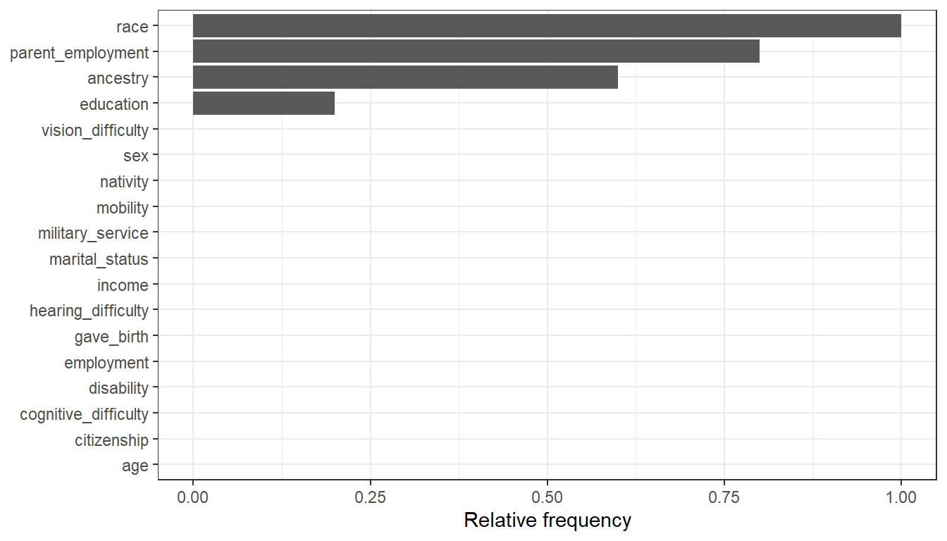
The frequency plot shows which features had to be changed most often to achieve the desired outcome. This tells us what the model is most sensitive to for this individual.

cfactuals$plot_freq_of_feature_changes()

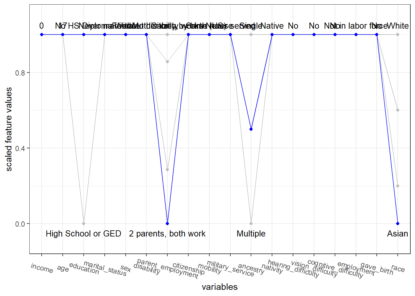
Finally, the parallel plot connects the feature values of each counterfactual (in black) and highlights our original person (person_of_interest) in blue. This makes it easy to see exactly what changed to flip the prediction (apparently graph is not optimized for many features..).

cfactuals$plot_parallel()

References

Biecek, Przemyslaw, and Tomasz Burzykowski. 2021. Explanatory Model Analysis: Explore, Explain, and Examine Predictive Models. Routledge Cavendish.

Molnar, Christoph. 2022. “Interpretable Machine Learning.” https://christophm.github.io/interpretable-ml-book/.

Footnotes

1. This makes them a great entry point for beginners and for communicating model-agnostic explainability to non-experts.

2. Attribution-based methods don’t show how sensitive the prediction is to local changes; CP plots do, completing the explanation.

3. They can be combined across models, classes, and features to create nuanced insights and are the basis for other interpretation methods.

4. This means we don’t automatically see how features interact, though manually changing two features is possible.

5. When features are correlated, some parts of the curve represent unlikely or unrealistic data points, which can be misleading.

6. This is a general problem, but the risk is higher for CP plots because their simplicity makes them easy to show to non-experts who may misinterpret them.