Appendix
1 R Example: Numeric outcome “income
This chapter walks through a full explainable AI and fairness audit for a regression task. We will train a Random Forest model to predict a person’s income and then use various techniques from the iml package to interpret its behavior.
1.1 1. Data Preparation and Splitting
First, we load the data, select our target variable income, and remove the old public_coverage variables. We then split the data into training and testing sets.
# Load and prepare data
data <- read_csv("data/data_acspubliccoverage.csv")
data <- data %>%
  mutate(across(where(is.character), as.factor)) %>%
  # Select income as the outcome and remove the old target variables
  select(income, everything(), -starts_with("public_coverage"))

# Split the data. For a numeric outcome, we can't use strata.
set.seed(123)
data_split <- initial_split(data, prop = 0.80)
data_train <- training(data_split)
data_test  <- testing(data_split)
1.2 2. Model Training
We define a tidymodels workflow to train a Random Forest model. The mode is now set to "regression" since income is a numeric outcome. The recipe includes steps to impute missing values and create dummy variables from factors.
# Define the recipe for a regression task
recipe_rf <- recipe(income ~ ., data = data_train) %>%
  step_impute_median(all_numeric_predictors()) %>%
  step_impute_mode(all_nominal_predictors()) %>%
  step_dummy(all_nominal_predictors(), one_hot = TRUE)

# Define a random forest model for REGRESSION
model_rf <- rand_forest(mode = "regression") %>%
  set_engine("ranger", importance = "impurity")

# Create and fit the workflow
workflow_rf <- workflow() %>%
  add_recipe(recipe_rf) %>%
  add_model(model_rf)
fit_rf <- fit(workflow_rf, data = data_train)
1.3 3. Model Evaluation
Before explaining the model, we check its performance on the test set using standard regression metrics like RMSE and R-squared. While the accuracy is not impressive we continue since the focus is on interpretability here.
# A tibble: 3 × 3
  .metric .estimator .estimate
  <chr>   <chr>          <dbl>
1 rmse    standard    7077.
2 rsq     standard       0.473
3 mae     standard    5327.
1.4 4. Global Feature Importance
1.4.1 Model-Specific Importance (Impurity)
We start by looking at the feature importance metric built into the Random Forest algorithm itself.
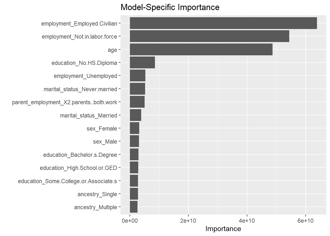
1.4.2 Model-Agnostic Permutation Importance
Next, we use the more robust method of Permutation Feature Importance (PFI) with the iml package. This measures how much the model’s error increases when a feature is shuffled.
# This function tells tidymodels to return a single numeric prediction
# and extracts the value from the ".pred" column.
p_fun_regression <- function(object, newdata) {
  predict(object, new_data = newdata, type = "numeric")$.pred
}

# First, create an iml Predictor object for the regression model
predictor <- Predictor$new(
  model = fit_rf,
  data = select(data_test, -income),
  y = data_test$income,
  predict.function = p_fun_regression,
  type = "regression"
)

# Calculate and plot permutation importance. The default loss for regression is RMSE.
pfi <- FeatureImp$new(predictor, loss = "rmse")
plot(pfi, n.features = 15)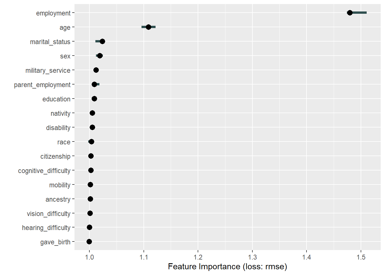
1.5 5. Global Feature Effects
1.5.1 PDP, ICE, and ALE Plots
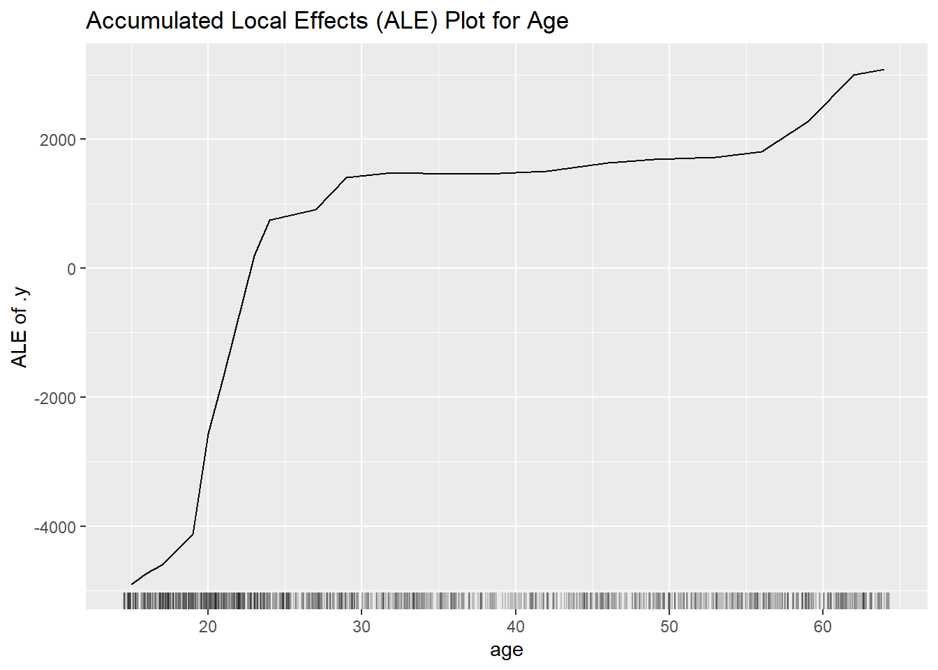
We can visualize how a feature affects the predicted income using Partial Dependence Plots (PDP), Individual Conditional Expectation (ICE) curves, and Accumulated Local Effects (ALE) plots.
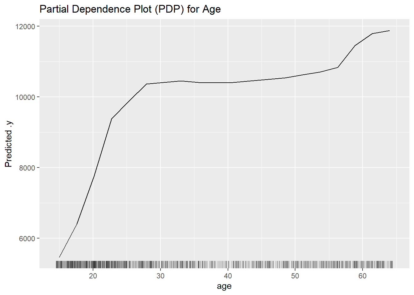
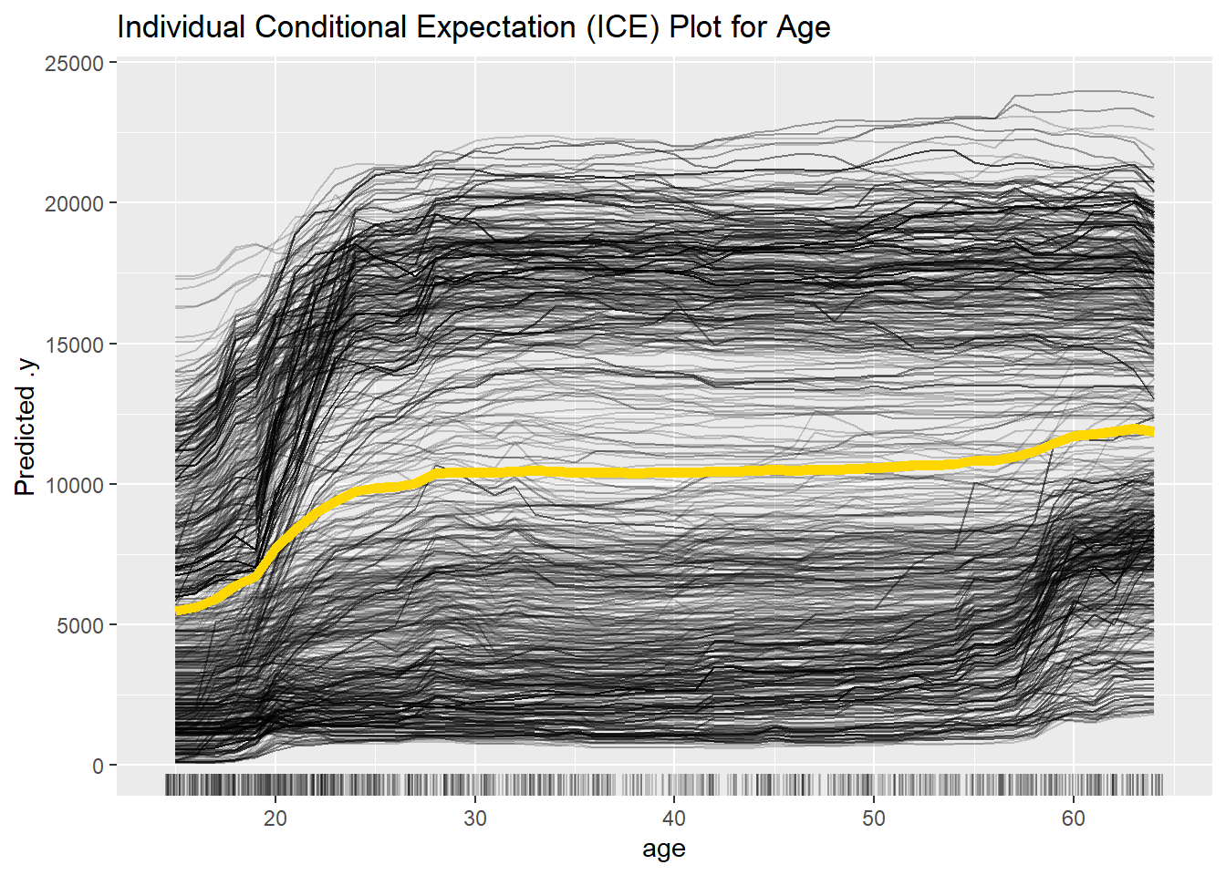
1.6 6. Interaction Strength
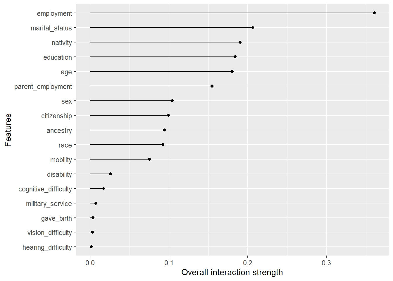
We can measure which features “team-up” the most by calculating Friedman’s H-statistic.
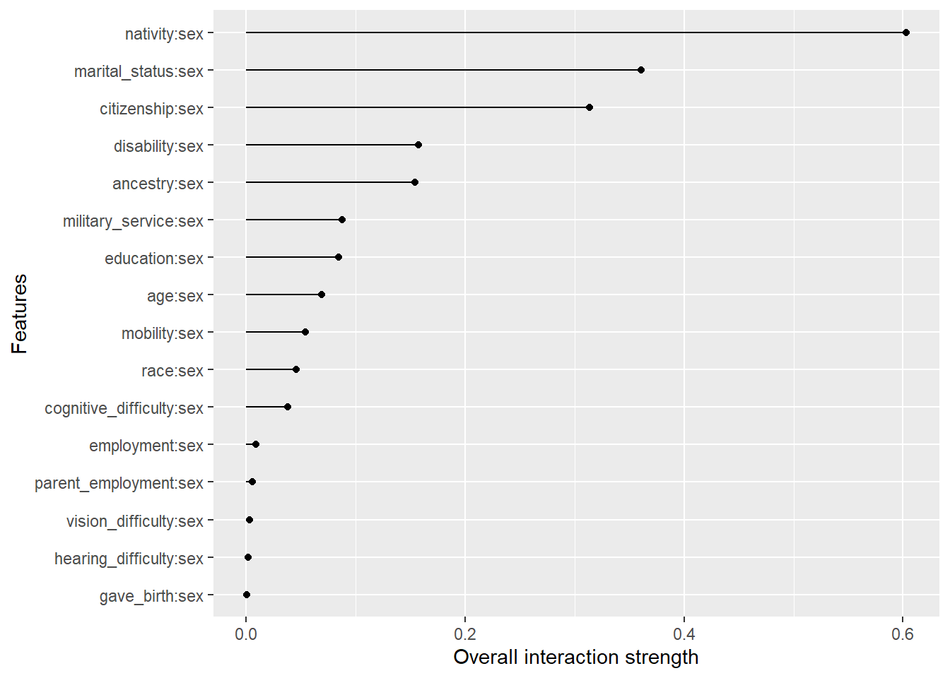
Let’s focus on the interactions specifically involving the sex feature.
1.7 7. Global Surrogate Model (LASSO)
We can train a simple, transparent LASSO model to mimic the behavior of our complex Random Forest. The important features in the LASSO model give us an approximation of what the Random Forest learned.
# --- Step 1: Get RF predictions on the training data ---
rf_predictions <- predict(fit_rf, new_data = data_train)$.pred
surrogate_train_data <- data_train %>%
  dplyr::select(-income) %>%
  mutate(rf_prediction = rf_predictions)

# --- Step 2: Train the LASSO Surrogate Model ---
lasso_spec <- linear_reg(penalty = tune(), mixture = 1) %>% set_engine("glmnet")
recipe_surrogate <- recipe(rf_prediction ~ ., data = surrogate_train_data) %>%
  step_impute_median(all_numeric_predictors()) %>%
  step_impute_mode(all_nominal_predictors()) %>%
  step_dummy(all_nominal_predictors(), one_hot = TRUE)

workflow_surrogate <- workflow() %>% add_recipe(recipe_surrogate) %>% add_model(lasso_spec)

# Tune and fit the surrogate model
set.seed(456)
folds <- vfold_cv(surrogate_train_data, v = 5)
lasso_tuned <- tune_grid(workflow_surrogate, resamples = folds, grid = 50)
best_penalty <- select_best(lasso_tuned, metric = "rmse")$penalty
fit_surrogate_final <- finalize_workflow(workflow_surrogate, list(penalty = best_penalty)) %>%
  fit(data = surrogate_train_data)

# --- Step 3: Interpret the Surrogate Model ---
vip(fit_surrogate_final, num_features = 15) +
  labs(title = "Global Surrogate (LASSO) Feature Importance")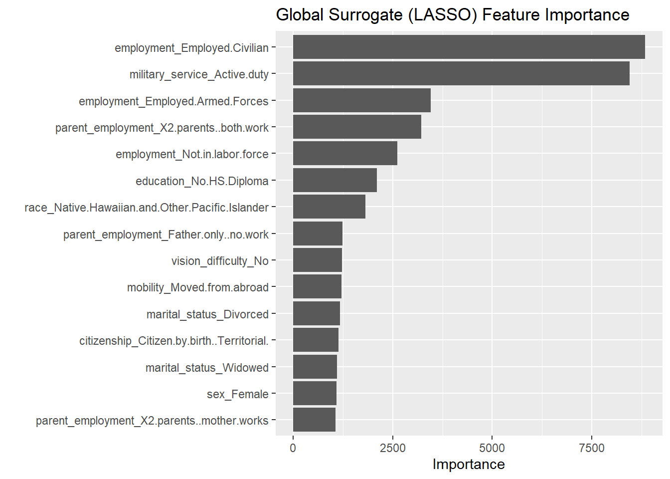
# --- Step 4: Measure Fidelity (R-squared) ---
test_preds_rf <- predict(fit_rf, new_data = data_test)$.pred
test_preds_surrogate <- predict(fit_surrogate_final, new_data = data_test)$.pred
fidelity <- rsq_vec(truth = test_preds_rf, estimate = test_preds_surrogate)
print(paste0("Surrogate Model Fidelity (R-squared): ", round(fidelity, 3)))
[1] "Surrogate Model Fidelity (R-squared): 0.813"