Feature Interaction

This chapter explains how to find and measure feature interactions, which occur when features work together to influence a model’s prediction.

Table 1: Selection of popular model-agnostic interpretation techniques, classified as local or global, and as effect or importance methods (Molnar et al. 2022).¹

Type	Local	Global
Feature Effects	Individual Conditional Expectation (ICE) Local Interpretable Model-Agnostic Explanations (LIME) Counterfactuals Shapley Values SHapley Additive exPlanation (SHAP)	Partial Dependence Plot (PDP) Accumulated Local Effects (ALE)
Feature Importance	Indivdual Conditional Importance (ICI)	Partial Importance (PI) Permutation Feature Importance (PFI) Shapley Additive Global Explanations (SAGE) H-Statistic*

*The H-statistic measures the overall interaction strength of a feature across the entire dataset, not for a single, specific prediction. This makes it a global method. It quantifies how much a feature’s interactions contribute to the model’s predictions. While it’s related to feature effects (it measures how effects change), its primary output is a single score representing the strength of these interactions, which aligns it more closely with feature importance methods.

1 Introduction: When Features Team Up

• Features often work together, not in isolation
• Effect of one feature depends on the value of another
• Combined effect is different than the sum of individual effects
• Fairness Risk: Interactions can create hidden bias against specific subgroups
  • e.g., unfair treatment for “women in engineering” even if the model is fair for men and women overall

2 Analogy: Sociology

• Analogy: A sociologist studies a job training program’s effect on employment.
  • Main effect: On average, the program increases employment.
  • Interaction effect: The program’s success depends on location. It’s highly effective in urban areas but has no effect in rural areas due to transportation issues.
  • Key Insight: The effect of the ‘program’ feature is not constant; it interacts with the ‘location’ feature.

3 Friedman and Popescu (2008)’s H-statistic

• A popular, model-agnostic metric
  • Measures feature “team-up” effects.
• Compares the combined effect of features vs. the sum of their individual effects.
• Goal: understand how much of the model’s prediction variance can be attributed to interactions between two specific features \(x_j, x_k\)
  • Decompose feature importance into main and interaction effects

4 The H-Statistic

• Intuition: Start with marginal effects of \(x_j, x_k\) without interaction²

\[ PD_{jk}(x_j, x_k) = PD_j(x_j) + PD_k(x_k) \]

• Compare variance of predictions of joint effect to variance of marginal effects³

\[ H^2_{jk} = \frac{\sum_{i=1}^n [PD_{jk}(x_j^{(i)}, x_k^{(i)}) - PD_j(x_j^{(i)}) - PD_k(x_k^{(i)})]^2}{\sum_{i=1}^n PD^2_{jk}(x_j^{(i)}, x_k^{(i)})} \]

• H-statistic formula is a ratio (similar to R-squared)
  • Tells us the proportion of the two-feature effect that can only be explained by their interaction
  • If \(H^2_{jk}\) is close to 0 → numerator is very small → interaction effect is weak → features are mostly additive
  • If \(H^2_{jk}\) is close to 1 → numerator is almost as large as denominator → combined effect is almost entirely driven by the interaction, not the individual features.

\[H^2_{jk} = \frac{\text{Variance Explained by Interaction}}{\text{Total Variance of the Joint Effect}}\]

5 Visualizing Feature Interaction (1)

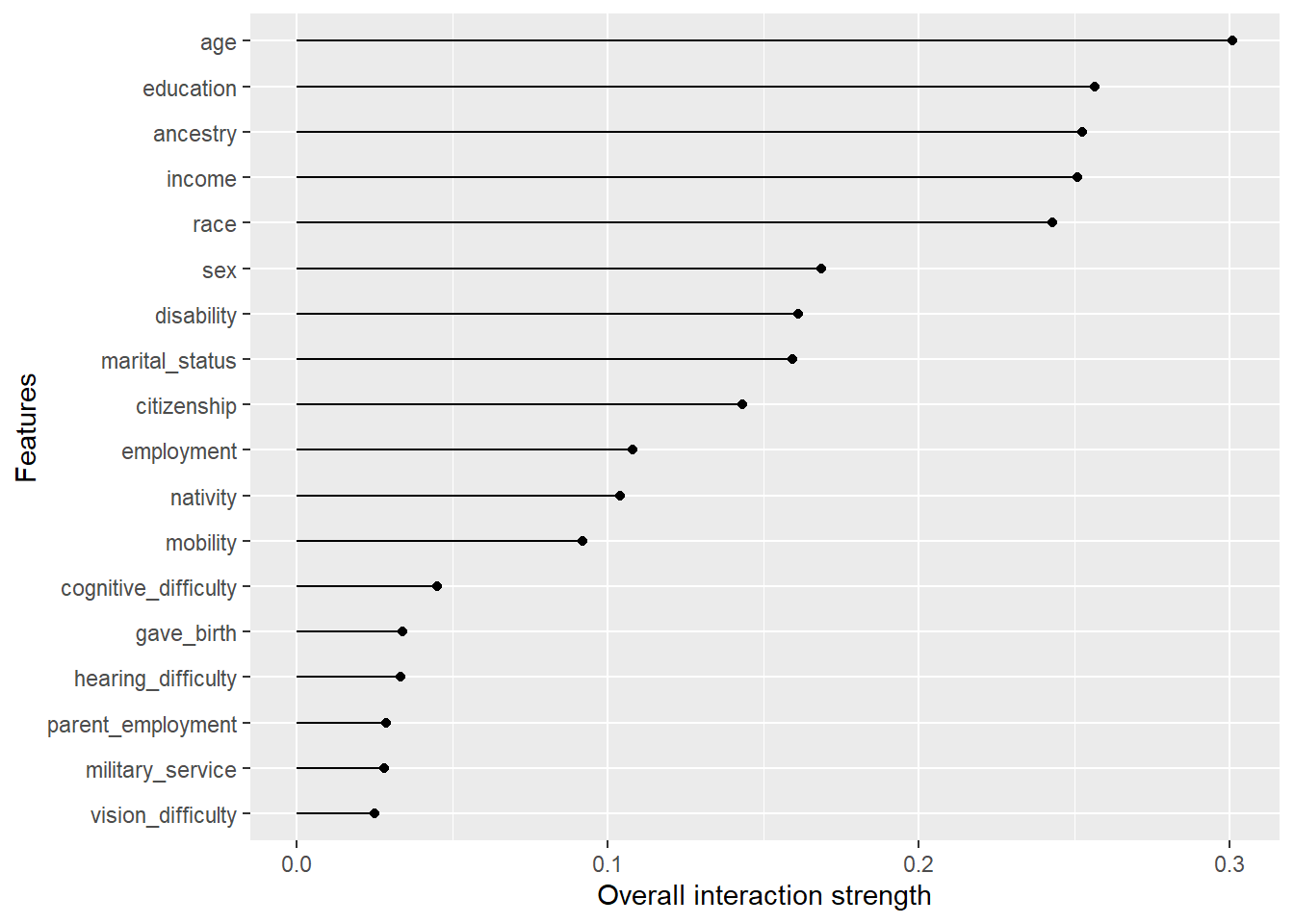
• Figure 1 shows overall interaction strength for each feature our model (Friedman’s H-statistic)
  • Score of e.g., 0.4 for variable \(X\) means that 43% of the variance in the model’s predictions that can be attributed to variable \(X\) is due to its interactions with all other features (“team players”)
  • High values = notable interaction effects → variables don’t work in isolation (Rules of thumb: \(< 0.1\): no worries; \(0.1 -0.4\): be cautios; \(> 0.4\): get worried)⁴
• e.g., age is one of the features with the strongest interaction effects⁵

Figure 1: Feature interaction measured through H-statistic

6 Visualizing Feature Interaction (2)

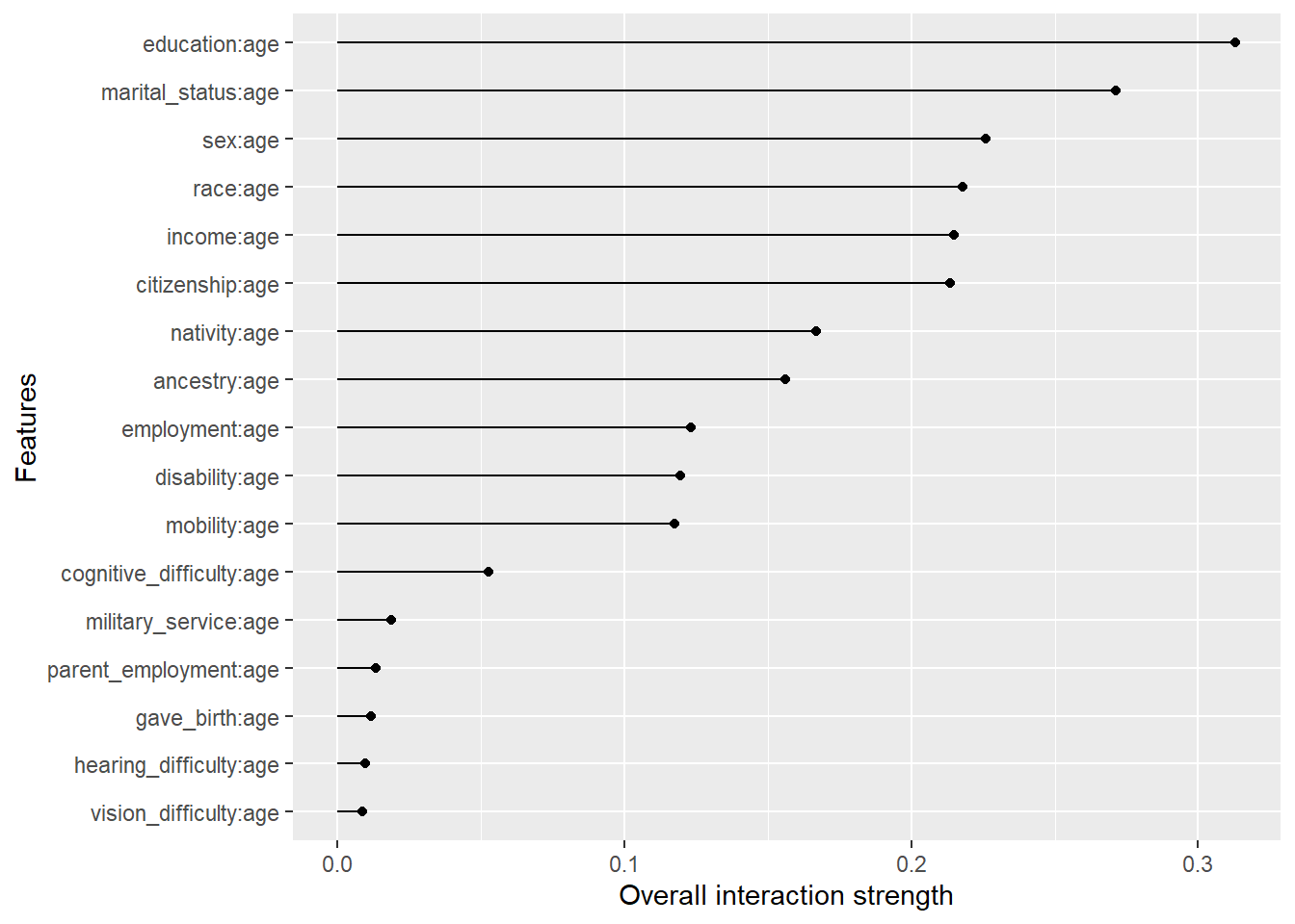
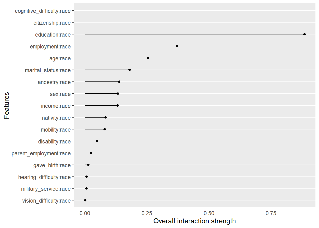
• Figure 2 shows the interaction strength between age and other variables. Do the results make sense?⁶

Figure 2: Feature interaction measured through H-statistic

7 Feature Interaction & Fairness (1)

• Interactions are a primary source of subgroup bias
• Problem: Model might seem fair on average, however, strong interaction could unfairly penalize a very specific group
• Example: A loan default model might use age and number_of_past_loans
  • The interaction could learn a spurious pattern that unfairly flags young applicants with few past loans as high-risk, even if each feature is fair on its own
• Audit workflow
  1. Check for important features.
  2. Calculate interaction strengths (H-statistic).
  3. Pay close attention to strong interactions, especially those involving sensitive or proxy features (can reveal hidden discrimination)

7.1 Strengths and Limitations: H-statistic

• Strengths
  • Backed by Theory⁷
  • Meaningful Interpretation⁸
  • Comparable⁹
  • Detects All Interaction Types¹⁰
  • Handles Higher-Order Interactions¹¹
• Limitations
  • Computationally Expensive¹²
  • Results Can Be Unstable¹³
  • No Model-Agnostic Significance Test¹⁴
  • Tells Strength, Not How¹⁵
  • Can Be Misleading (Spurious Interactions)¹⁶

8 Summary & Key Takeaways

• Feature interactions occur when combined effect of features differs from their individual effects
• H-statistic is a powerful tool to measure strength of these interactions
• Analyzing interactions is a crucial step in fairness audits (subgroup biases related to interactions)
• Investigate strong interactions that involve sensitive attributes/proxies

9 Lab R: Uncovering Interactions

This lab uses our trained model for predicting public health coverage to find the strongest feature interactions. Understanding interactions is a key step in advanced fairness audits, as they can reveal biases that affect specific subgroups.

• Goal: Calculate Friedman’s H-statistic for feature pairs and analyze them for potential fairness issues.
• R Libraries: tidymodels, iml

9.1 Prepare data and train model

Before we can find interactions, we need a trained model. We can reuse the tidymodels workflow from the previous exercise. For completeness, the setup code is included again here.

library(tidymodels)
library(iml)
library(dplyr)
library(tidyverse)

#data <- read_csv(url(sprintf("https://docs.google.com/uc?id=%s&export=download",
#                         "1dnCK79T45Qa7RZrDg1qv6-EdGBoxCPjv")))

data <- read_csv("data/data_acspubliccoverage.csv")
data <- data %>% mutate(across(where(is.character), as.factor))

# Split the clean data
set.seed(123)
data_split <- initial_split(data, prop = 0.80, strata = public_coverage)
data_train <- training(data_split)
data_test  <- testing(data_split)

# Define the recipe and model spec
recipe_rf <- recipe(public_coverage ~ ., data = data_train)
model_rf <- rand_forest(mode = "classification") %>% set_engine("ranger")

# Create and fit the workflow
workflow_rf <- workflow() %>%
  add_recipe(recipe_rf) %>%
  add_model(model_rf)
fit_rf <- fit(workflow_rf, data = data_train)

9.2 Create an iml Predictor Object

The iml package, which calculates interactions, needs its own “predictor” object to wrap our tidymodels workflow. We’ll create that now.

# iml needs a custom function to get prediction probabilities from a tidymodels workflow
predict_fun <- function(model, newdata) {
  predict(model, new_data = newdata, type = "prob")$.pred_Yes
}

# Create the predictor object
# We use the training data to build the explainer
predictor <- iml::Predictor$new(
  model = fit_rf,
  data = select(data_train, -public_coverage),
  y = data_train$public_coverage == "Yes",
  predict.function = predict_fun
)

9.3 Task 1: Calculate Overall Interaction Strength

• Instructions: Use iml::Interaction$new() to calculate the interaction strengths. This can be computationally intensive, so be patient. Then, plot the results to see the top interactions.
  • grid.size: is the random sample of data points that the algorithm uses to perform its calculations (the higher the better)
• Discussion Question: What are the top interactions? Does it make intuitive sense that these features would work together to predict the need for public health coverage? (e.g., the effect of income might be different depending on a person’s age).

# Detect cores
  library(parallel)
  detectCores()

[1] 22

library("future")
library("future.callr")
# Use several cores
plan("callr", workers = 4)

# This step can take a few minutes to run!
interactions <- iml::Interaction$new(predictor, grid.size = 100) # Pick values > 100 better >1000

# Plot the results to see the strongest interactions
plot(interactions)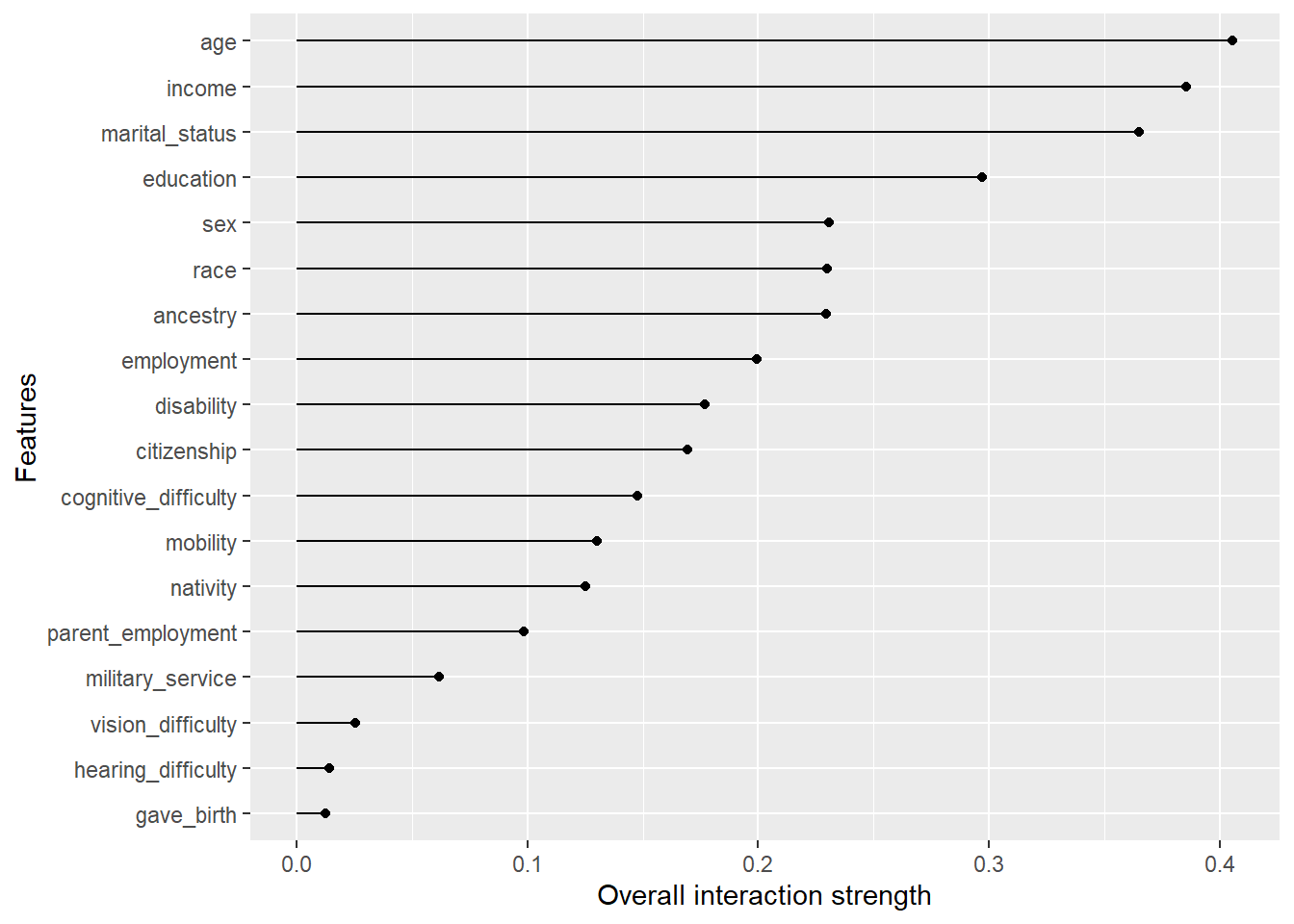

Top feature interactions based on Friedman’s H-statistic.

9.4 Task 2: Fairness Investigation

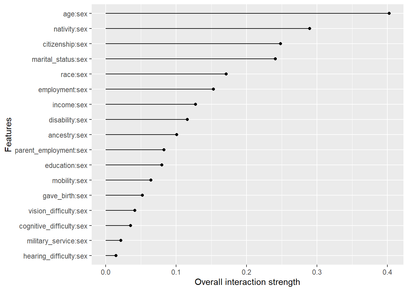
Let’s specifically check for interactions involving one of our protected attributes: sex. A strong interaction with a protected attribute can be a sign of subgroup bias, where the model treats combinations of features differently for different groups.

• Instructions: We can focus the analysis on a single feature. Let’s create a plot showing the interaction strength between sex and all other features.
• Critical Thinking: Look at the plot. What are the strongest interactions involving sex? If you see a strong interaction (e.g., between sex and marital_status), what does that mean? It suggests the model’s interpretation of marital status is different for men than for women, which is a sign of potential subgroup bias that requires further investigation.

plan("callr", workers = 4)

interactions_sex <- iml::Interaction$new(predictor, feature = "sex", 
                                         grid.size = 100)  # Pick values > 100 better >1000

# Plot the results
plot(interactions_sex)

Interaction strengths for the ‘sex’ feature.

9.5 Exercise R

1. Please use the code below.
2. Start by exploring overall interaction strength (simply rerun the code from above).
3. Then explore the feature race and try to find out with which other features it displays the strongest interaction.
   • How would you interpret the results?

library(tidymodels)
library(iml)
library(dplyr)
library(tidyverse)

#data <- read_csv(url(sprintf("https://docs.google.com/uc?id=%s&export=download",
#                         "1dnCK79T45Qa7RZrDg1qv6-EdGBoxCPjv")))

data <- read_csv("data/data_acspubliccoverage.csv")
data <- data %>% mutate(across(where(is.character), as.factor))

# Split the clean data
set.seed(123)
data_split <- initial_split(data, prop = 0.80, strata = public_coverage)
data_train <- training(data_split)
data_test  <- testing(data_split)

# Define the recipe and model spec
recipe_rf <- recipe(public_coverage ~ ., data = data_train)
model_rf <- rand_forest(mode = "classification") %>% set_engine("ranger")

# Create and fit the workflow
workflow_rf <- workflow() %>%
  add_recipe(recipe_rf) %>%
  add_model(model_rf)
fit_rf <- fit(workflow_rf, data = data_train)

# iml needs a custom function to get prediction probabilities from a tidymodels workflow
predict_fun <- function(model, newdata) {
  predict(model, new_data = newdata, type = "prob")$.pred_Yes
}

# Create the predictor object
# We use the training data to build the explainer
predictor <- iml::Predictor$new(
  model = fit_rf,
  data = select(data_train, -public_coverage),
  y = data_train$public_coverage == "Yes",
  predict.function = predict_fun
)

Answer/Solution(s)

# Detect cores
  library(parallel)
  detectCores()

[1] 22

library("future")
library("future.callr")
# Use several cores
plan("callr", workers = 10)

# This step can take a few minutes to run!
interactions <- iml::Interaction$new(predictor, grid.size = 10)

# Plot the results to see the strongest interactions
plot(interactions)

Top feature interactions based on Friedman’s H-statistic.

plan("callr", workers = 10)

interactions_sex <- iml::Interaction$new(predictor, feature = "race", 
                                         grid.size = 5)

# Plot the results
plot(interactions_sex)

Interaction strengths for the ‘sex’ feature.

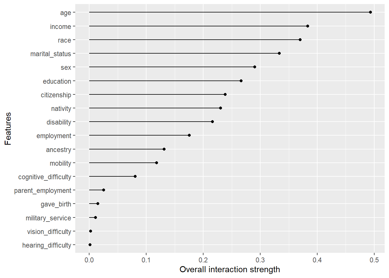
10 Lab Python

Overview: https://docs.google.com/document/d/1mUDDwZMZR-9aRZhvSzDEC85sXmwOMB4Y8okMXbehytY/

References

Friedman, Jerome H, and Bogdan E Popescu. 2008. “Predictive Learning via Rule Ensembles.” The Annals of Applied Statistics 2 (3): 916–54.

Molnar, Christoph, Gunnar König, Julia Herbinger, Timo Freiesleben, Susanne Dandl, Christian A Scholbeck, Giuseppe Casalicchio, Moritz Grosse-Wentrup, and Bernd Bischl. 2022. “General Pitfalls of Model-Agnostic Interpretation Methods for Machine Learning Models.” In xxAI - Beyond Explainable AI, 39–68. Springer International Publishing.

Footnotes

1. Global interpretation methods: describe the expected behavior of the entire model with respect to the whole data distribution. Local explanation methods: explain individual predictions or classifications. Feature importance methods: quantify the contribution of a feature to the model performance (e.g. via a loss function) or to the variance of the prediction function. Effect methods: indicate the direction and magnitude of a change in predicted outcome due to changes in feature values (Molnar et al. 2022, 40–41).

2. The formula below describes a hypothetical, perfect world with zero interaction. It acts as our baseline for comparison. PD stands for Partial Dependence. \(PD_j(x_j)\) is the average effect of feature j on the model’s prediction. \(PD_k(x_k)\) is the average effect of feature k on the prediction. \(PD_{jk}(x_j, x_k)\) is the average effect of features j and k working together. What does the formula say? It describes a simple world where the combined effect of two features is just the sum of their individual effects. For example, if increasing age adds 0.1 to the prediction and increasing income adds 0.2, their combined effect would be exactly 0.3. The H-statistic works by measuring how much our real model deviates from this simple, additive assumption.

3. The formula below calculates the proportion of the joint effect’s variance that is explained by the interaction. The numerator sums up the squared differences between the actual joint effect and the hypothetical “no-interaction” effect across all data points (e.g., all individuals). The term inside the brackets, \(PD_{jk} - (PD_j + PD_k)\), is the interaction effect for a single data point. By squaring and summing these values, the numerator represents the total variance of the model’s predictions that is due only to the interaction. The denominator sums the squared joint effects across all data points. This represents the total variance of the model’s predictions that is due to the two features working together.

4. Importantly, there is no single “correct” threshold. However, when the H-statistic is very high ideally stop looking at 1D PDPs, try 2D PDP.

5. Meaning a significant portion of its predictive power comes from how it combines with other variables and the model’s interpretation of other features likely changes depending on a person’s age.

6. Interpretation: The effect of a person’s income on their predicted public insurace coverage status is not constant; it changes significantly based on their employment status and educational background.

7. The interaction H-statistic has an underlying theory through the partial dependence decomposition.

8. The interaction is defined as the share of variance that is explained by the interaction.

9. Since the statistic is dimensionless, it is comparable across features and even across different models.

10. The statistic detects all kinds of interactions, regardless of their particular form.

11. It’s possible to analyze arbitrary higher-order interactions, such as the strength between 3 or more features.

12. The first thing you will notice: The interaction H-statistic takes a long time to compute.

13. The computation involves estimating marginal distributions, which have a certain variance. This means results can vary from run to run, especially with smaller samples.

14. It’s unclear whether an interaction is significantly greater than 0. We would need a statistical test, but this is not (yet) available in a model-agnostic version.

15. The H-statistic tells us the strength of an interaction, but it does not tell us how the interaction looks. You still need Partial Dependence Plots for that.

16. If the total effect of two features is weak but consists mostly of interaction, the H-statistic can be very large. This can cause a spurious interaction to be over-interpreted as strong.