| Type | Local | Global |
|---|---|---|
| Feature Effects |
|
|
| Feature Importance |
|
|
Local Interpretable Model-Agnostic Explanations (LIME) & Surrogate models
This chapter covers surrogate models, which are simple, interpretable models trained to explain a more complex “black box” model. We’ll focus on LIME for local, single-prediction explanations and the broader concept of global surrogates.
1 Introduction: Explaining the Unexplainable
- Complex models are often “black boxes”; we don’t know why they make a specific decision
- Problem: How to explain a single prediction (e.g., “Why was this loan denied?”)
- Solution: Use a simple, transparent surrogate model to approximate the complex one’s behavior
- Analogy: Approximating one curve on a complex, winding road with a simple, straight line
- Q: What models are simple again?
2 Local vs. Global Surrogates
- LIME: Local Interpretable Model-agnostic Explanations
- Tool that finds simple “straight line” to explain one specific point, a single prediction
- Global surrogate
- like trying to approximate the entire winding road with a simpler map of just a few key turns.
3 LIME (Local Interpretable Model-agnostic Explanations)
- Creates a simple, local model to explain one prediction at a time (cf. Ribeiro, Singh, and Guestrin 2016)
- Approximates complex model’s behavior only in “neighborhood” of instance you want to explain.
- How LIME Works:
- Select your instance of interest2 for which you want to have an explanation of its black box prediction.
- Perturb your dataset3 and get the black box predictions for these new points.
- Weight the new samples according to their proximity to the instance of interest.
- Train a weighted, interpretable model on the dataset with the variations.
- Explain the prediction by interpreting the local model.
4 LIME Intuition
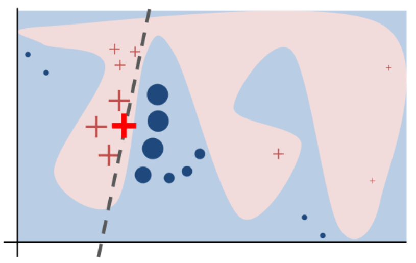
5 LIME plot
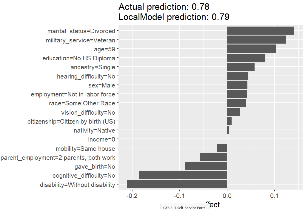
- Interpretation of “Lime plot” in Figure 1 (you pick number of features)
- Actual prediction = original predicted probability by random forest
- LocalModel prediction = predicted probability by simple, local linear model that LIME created5
- Bars to the left (Negative Effect): These feature values push the prediction DOWN6
- Bars to the right (Positive Effect): These features push the prediction UP7
- bars = coefficients of linear model reflecting difference to the average predicted probability
- 0-line = intercept = average predicted probability
- labels, e.g., age (feature) = 59 (feature value of the current individual)
6 Strengths and Limitations: LIME
7 Global Surrogate Models
- General idea: Approximate
black boxmodel with a simpler model (cf. e.g., Craven and Shavlik 1995)- Train simple, transparent model (e.g., a decision tree) to mimic entire black box model’s behavior
- How it Works:
- Get the predictions from the black box model for your dataset.
- Train a simple, interpretable model (e.g., decision tree or lasso) to predict the black box’s predictions (not the original true labels).
- If the surrogate model is accurate, its simple logic provides a good approximation of the complex model’s overall behavior.
- Caveat: The surrogate is only an approximation and may not capture all the nuance of the original, more complex model.
8 Surrogates and Fairness
Powerful tools for auditing bias at both the individual and systemic levels.
LIME for Individual Fairness
- Debugs single, potentially biased outcomes.
- Shows if a decision was based on legitimate factors or proxies for protected attributes (e.g., race, sex).
- Answers the crucial question: “Why was I treated this way?”, which is fundamental for providing recourse.
Global Surrogates for Systemic Bias
- Reveals the overall “rules of thumb” the complex model has learned.
- A decision tree surrogate can uncover discriminatory system-level patterns, such as rules based on
zip_codethat act as a proxy for race.
9 Summary & Key Takeaways
- Surrogate models: Simple models used to explain complex black boxes.
- LIME: A local surrogate; explains one prediction at a time.
- Global surrogates: A global surrogate; mimics the entire model’s behavior.
- LIME for Fairness: Critical for individual accountability and debugging specific unfair outcomes.
- Global Surrogates for Fairness: Reveal overall model logic and can uncover systemic biases.
10 Lab R: Explaining Predictions with LIME
- We will use our trained income prediction model to explain why it makes certain decisions for specific individuals.
- Goal: Use LIME to generate and interpret local explanations.
- R Library: iml
10.1 Prepare data and train model
First, we’ll run the setup code to train our Random Forest model.
library(tidymodels)
library(iml) # Use iml instead of DALEX
library(dplyr)
library(readr)

# Load and prepare data
#data <- read_csv(url(sprintf("https://docs.google.com/uc?id=%s&export=download",
#                         "1dnCK79T45Qa7RZrDg1qv6-EdGBoxCPjv")))
data <- read_csv("data/data_acspubliccoverage.csv")
data <- data %>% mutate(across(where(is.character), as.factor))

# Split the data
set.seed(123)
data_split <- initial_split(data, prop = 0.80, strata = public_coverage)
data_train <- training(data_split)
data_test  <- testing(data_split)

# Define the recipe and model spec
recipe_rf <- recipe(public_coverage ~ ., data = data_train)%>%
  step_impute_median(all_numeric_predictors()) %>% # Impute numeric NAs
  step_impute_mode(all_nominal_predictors())      # Impute categorical NAs
model_rf <- rand_forest(mode = "classification") %>% set_engine("ranger")

# Create and fit the workflow
workflow_rf <- workflow() %>%
  add_recipe(recipe_rf) %>%
  add_model(model_rf)
fit_rf <- fit(workflow_rf, data = data_train)
10.2 Create explainer
Then, we will create an iml Predictor object, which is necessary for generating explanations. Here we bake our data_test to obtain baked_test_data, i.e., we prepare the recipe_rf and apply it to data_test as to make sure that baked_test_data was put through all the data preprocessing steps.
# Before creating the predictor, we need to "bake" the test data.
# This applies the trained recipe (including imputation) to the test set.
prepped_recipe <- prep(recipe_rf, training = data_train)
baked_test_data <- bake(prepped_recipe, new_data = data_test)

# --- Create the iml Predictor Object ---
# This object wraps the model and data for the iml package
p_fun <- function(object, newdata) {
  predict(object, new_data = newdata, type = "prob")$.pred_Yes
}

predictor <- Predictor$new(
  model = fit_rf,
  data = select(baked_test_data, -public_coverage), # Predictor variables from test set
  y = baked_test_data$public_coverage,              # Outcome variable from test set
  predict.function = p_fun,
  type = "classification"                     # Specify the task type
)
10.3 Task 1: Explain a Correct Prediction
- Instructions: Find a person in your test set that the model correctly predicted would have public insurance coverage. Generate a LIME explanation plot for this individual using
iml. - Discussion Question: Which features did LIME identify as supporting or opposing the “Yes” prediction? Do these features make intuitive sense?16
# First, get predictions for the test set to find a correct instance
predictions <- augment(x = fit_rf, new_data = baked_test_data)

# Find one person who was correctly predicted to have public coverage
correct_yes_case <- predictions %>%
  filter(public_coverage == "Yes" & .pred_class == "Yes") %>%
  drop_na() %>%
  # LIME needs only the predictor columns
  select(all_of(predictor$data$feature.names)) %>%
  slice(1)

# Generate the LIME explanation for this single case using iml's LocalModel
lime_correct <- LocalModel$new(
  predictor = predictor,
  x.interest = correct_yes_case,
  k = 18 # Specify the number of features to show in the explanation
)

# Plot the explanation
plot(lime_correct)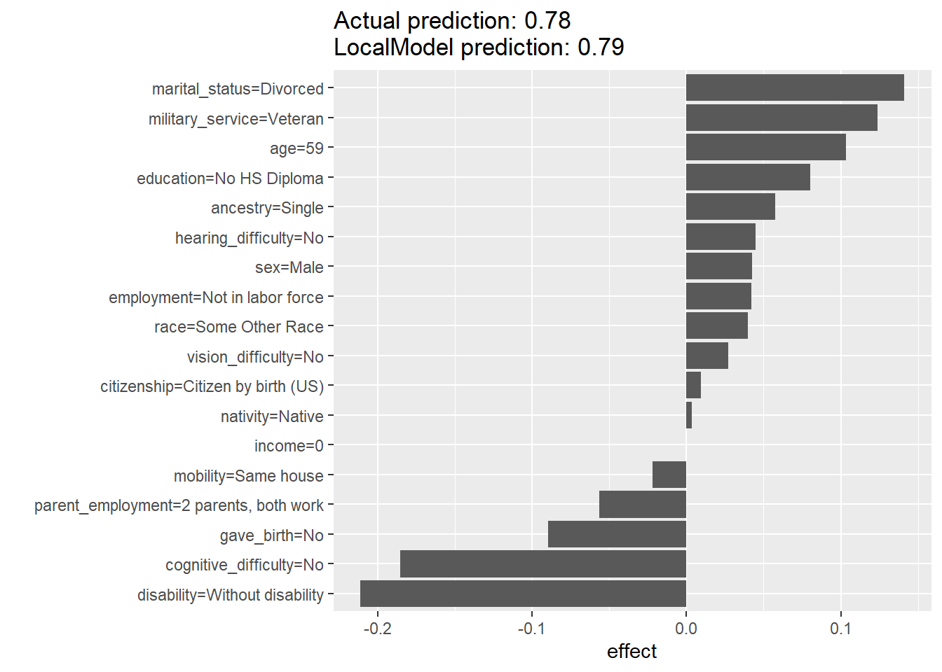
10.4 Task 2: Explain an Incorrect Prediction
- Instructions: Now, find a person for whom the model made a mistake. Generate the LIME explanation for this case.
- Discussion Question: Can LIME help you understand why the model was wrong? Perhaps it put too much weight on a misleading feature for this specific person.
# Find one person who was incorrectly predicted as "No"
incorrect_case <- predictions %>%
  filter(public_coverage == "Yes" & .pred_class == "No") %>%
  drop_na() %>%
  select(all_of(predictor$data$feature.names)) %>%
  slice(1)

# Generate the LIME explanation
lime_incorrect <- LocalModel$new(
  predictor = predictor,
  x.interest = incorrect_case,
  k = 18 # Specify the number of features to show in the explanation
)

plot(lime_incorrect)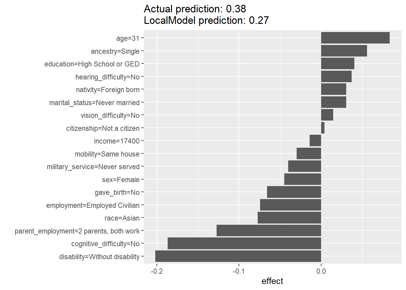
10.5 Task 3: Fairness Investigation
- Instructions: Find two individuals who are similar in most respects but differ in the sensitive attribute
sex. Generate LIME explanations for both. - Critical Thinking: Compare the two explanations. Does the model use the same logic for both people? Does
sexappear as an important feature in either explanation? This is a direct way to probe the model for individual-level bias.
# Find two similar people who differ by sex.
similar_pair <- baked_test_data %>%
  filter(income<18000, income>6200, education == "Bachelor's Degree") %>%
  # Find one male and one female from this group
  group_by(sex) %>%
  slice(1) %>%
  ungroup()

# Isolate the two observations
person_1 <- similar_pair %>% slice(1) %>% select(all_of(predictor$data$feature.names))
person_2 <- similar_pair %>% slice(2) %>% select(all_of(predictor$data$feature.names))

# Generate explanations for both
lime_person_1 <- LocalModel$new(predictor = predictor, x.interest = person_1, k = 18)
lime_person_2 <- LocalModel$new(predictor = predictor, x.interest = person_2, k = 18)

# The plot function in iml can accept multiple explanation objects to compare them
plot(lime_person_1)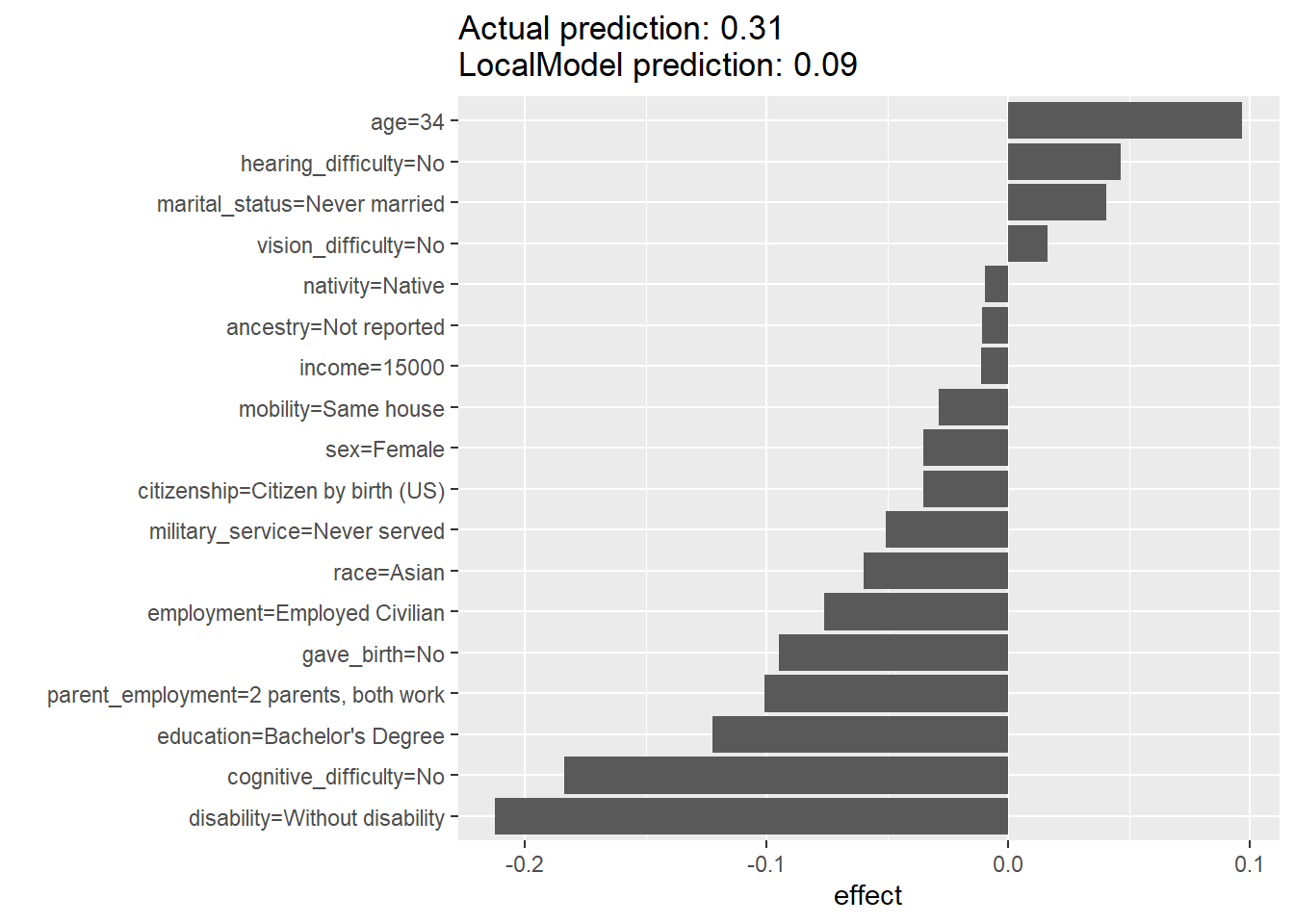
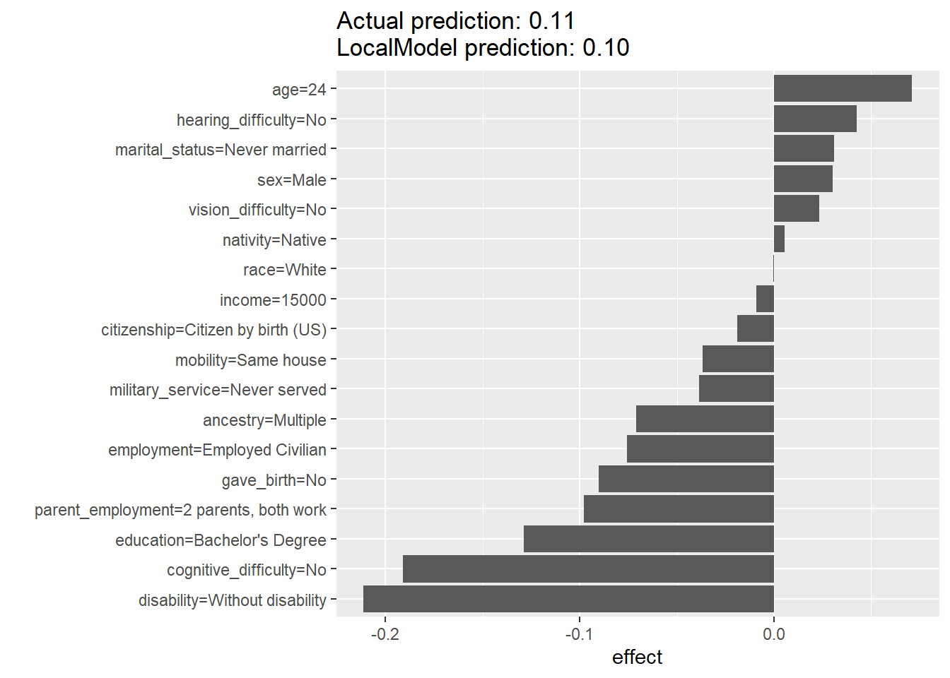
10.6 Exercise R
- Please use the code below (and above), pick an individual from the test dataset (either of class 0 = no public coverage or 1 = public coverage) and explain the corresponding prediction using lime. The code below may help.
library(tidymodels)
library(iml) # Use iml instead of DALEX
library(dplyr)
library(readr)

# Load and prepare data
#data <- read_csv(url(sprintf("https://docs.google.com/uc?id=%s&export=download",
#                         "1dnCK79T45Qa7RZrDg1qv6-EdGBoxCPjv")))
data <- read_csv("data/data_acspubliccoverage.csv")
data <- data %>% mutate(across(where(is.character), as.factor))

# Split the data
set.seed(123)
data_split <- initial_split(data, prop = 0.80, strata = public_coverage)
data_train <- training(data_split)
data_test  <- testing(data_split)

# Define the recipe and model spec
recipe_rf <- recipe(public_coverage ~ ., data = data_train)%>%
  step_impute_median(all_numeric_predictors()) %>% # Impute numeric NAs
  step_impute_mode(all_nominal_predictors())      # Impute categorical NAs
model_rf <- rand_forest(mode = "classification") %>% set_engine("ranger")

# Create and fit the workflow
workflow_rf <- workflow() %>%
  add_recipe(recipe_rf) %>%
  add_model(model_rf)
fit_rf <- fit(workflow_rf, data = data_train)
# Before creating the predictor, we need to "bake" the test data.
# This applies the trained recipe (including imputation) to the test set.
prepped_recipe <- prep(recipe_rf, training = data_train)
baked_test_data <- bake(prepped_recipe, new_data = data_test)
# --- Create the iml Predictor Object ---
# This object wraps the model and data for the iml package
p_fun <- function(object, newdata) {
predict(object, new_data = newdata, type = "prob")$.pred_Yes
}
predictor <- Predictor$new(
model = fit_rf,
data = select(baked_test_data, -public_coverage), # Predictor variables from test set
y = baked_test_data$public_coverage, # Outcome variable from test set
predict.function = p_fun,
type = "classification" # Specify the task type
)# First, get predictions for the test set to find a correct instance
predictions <- augment(x = fit_rf, new_data = baked_test_data)
# Find one person who was correctly predicted to have public coverage
correct_yes_case <- predictions %>%
filter(public_coverage == "Yes" & .pred_class == "Yes") %>%
drop_na() %>%
# LIME needs only the predictor columns
select(all_of(predictor$data$feature.names)) %>%
slice(1)
# Generate the LIME explanation for this single case using iml's LocalModel
lime_correct <- LocalModel$new(
predictor = predictor,
x.interest = correct_yes_case,
k = 18 # Specify the number of features to show in the explanation
)
# Plot the explanation
plot(lime_correct)11 Lab R: Global Surrogate Model
This document demonstrates how to train a LASSO model as a global surrogate to explain a more complex Random Forest model using the tidymodels package.
11.1 Train the Black Box Model
First, we’ll run your setup code to train the Random Forest model. This is our “black box” model that we want to explain.
library(tidymodels)
library(iml)
library(dplyr)
library(readr)
library(glmnet) # For LASSO model

# Load and prepare data
#data <- read_csv(url(sprintf("https://docs.google.com/uc?id=%s&export=download",
#                         "1dnCK79T45Qa7RZrDg1qv6-EdGBoxCPjv")))
data <- read_csv("data/data_acspubliccoverage.csv")
data <- data %>% mutate(across(where(is.character), as.factor))

# Split the data
set.seed(123)
data_split <- initial_split(data, prop = 0.80, strata = public_coverage)
data_train <- training(data_split)
data_test  <- testing(data_split)

# Define the recipe and model spec for the Random Forest
recipe_rf <- recipe(public_coverage ~ ., data = data_train) %>%
  step_impute_median(all_numeric_predictors()) %>%
  step_impute_mode(all_nominal_predictors()) %>%
  step_dummy(all_nominal_predictors(), one_hot = TRUE) # one_hot encoding for LASSO

model_rf <- rand_forest(mode = "classification") %>% set_engine("ranger", importance = "impurity")

# Create and fit the workflow
workflow_rf <- workflow() %>%
  add_recipe(recipe_rf) %>%
  add_model(model_rf)
fit_rf <- fit(workflow_rf, data = data_train)

vip(fit_rf, num_features = 15) +
  labs(title = "Global Surrogate (LASSO) Feature Importance")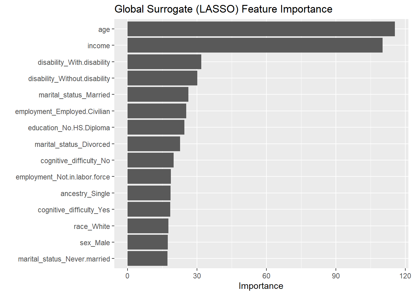
11.2 Train the LASSO Surrogate Model
The core idea of a surrogate model is to train a simple model to predict the outputs of the complex model.
- Get Predictions: We’ll use our trained Random Forest to get probability predictions for the training data.
- Train LASSO: We’ll then train a LASSO model using the original features to predict these probabilities.
# --- Step 1: Get Predictions from the Black Box Model ---
# The surrogate model will learn to mimic these probabilities.
rf_predictions <- predict(fit_rf, new_data = data_train, type = "prob")
# Important: fit_rf contains the recipe

# Prepare the training data for the surrogate
# The outcome is now the RF's predicted probability for "Yes"
data_train_surrogate <- data_train %>%
  select(-public_coverage) %>%
  bind_cols(rf_predictions) %>%
  select(-.pred_No)


# --- Step 2: Train the LASSO Surrogate Model ---
# We define a LASSO model spec (mixture = 1 means it's a LASSO)
# We need to tune the penalty (lambda) to find the best value.
model_surrogate <- linear_reg(penalty = tune(), mixture = 1) %>%
  set_engine("glmnet")

# The recipe is the same, but the outcome is now .pred_Yes
recipe_surrogate <- recipe(.pred_Yes ~ ., data = data_train_surrogate) %>%
  step_impute_median(all_numeric_predictors()) %>%
  step_impute_mode(all_nominal_predictors()) %>%
  step_dummy(all_nominal_predictors(), one_hot = TRUE)

# Create a workflow for the surrogate model
workflow_surrogate <- workflow() %>%
  add_recipe(recipe_surrogate) %>%
  add_model(model_surrogate)

# Tune the penalty parameter to find the best LASSO model
set.seed(456)
folds <- vfold_cv(data_train_surrogate, v = 5)
lasso_grid <- grid_regular(penalty(), levels = 50)

lasso_tuned <- tune_grid(
  workflow_surrogate,
  resamples = folds,
  grid = lasso_grid
)

# Finalize the workflow with the best penalty and fit the final surrogate model
best_penalty <- select_best(lasso_tuned, metric = "rmse")$penalty

worflow_final_surrogate <- finalize_workflow(workflow_surrogate,
                                             list(penalty = best_penalty))

fit_surrogate_final <- fit(worflow_final_surrogate,
                           data = data_train_surrogate)
11.3 Interpret the Surrogate Model
Now that we have our trained LASSO surrogate, we can interpret it. The features with non-zero coefficients are the ones the Random Forest implicitly learned were most important.
# A tibble: 62 × 3
   term                                       estimate  penalty
   <chr>                                         <dbl>    <dbl>
 1 (Intercept)                                  0.464  0.000869
 2 military_service_Veteran                     0.212  0.000869
 3 disability_With.disability                   0.212  0.000869
 4 parent_employment_Mother.only..no.work       0.164  0.000869
 5 marital_status_Divorced                      0.123  0.000869
 6 race_Black.or.African.American               0.102  0.000869
 7 education_No.HS.Diploma                      0.0999 0.000869
 8 parent_employment_X2.parents..mother.works   0.0942 0.000869
 9 marital_status_Widowed                       0.0932 0.000869
10 employment_Unemployed                        0.0750 0.000869
# ℹ 52 more rows
Besides, we can estimate feature importance statistics for the Lasso’s features.
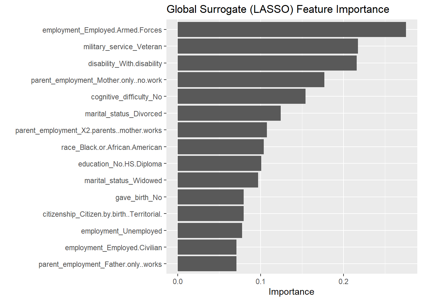
11.3.1 Measuring Fidelity
Finally, we need to check how well our simple LASSO model actually mimics the complex Random Forest. We measure this with R-squared, which tells us how much of the variance in the Random Forest’s predictions is captured by the LASSO model. A high R-squared (e.g., > 0.8) means we have a high-fidelity surrogate.
# Get predictions from both models on the test set
rf_test_preds <- predict(fit_rf, new_data = data_test, type = "prob")$.pred_Yes

surrogate_test_preds <- predict(fit_surrogate_final, new_data = data_test)$.pred

# Calculate R-squared between the two sets of predictions
fidelity <- rsq_vec(
  truth = rf_test_preds,
  estimate = surrogate_test_preds
)

print(paste0("Surrogate Model Fidelity (R-squared): ", round(fidelity, 3)))
[1] "Surrogate Model Fidelity (R-squared): 0.694"12 Lab Python
Overview: https://docs.google.com/document/d/1mUDDwZMZR-9aRZhvSzDEC85sXmwOMB4Y8okMXbehytY/
13 Appendix
Craven, Mark W, and Jude W Shavlik. 1995. “Extracting Tree-Structured Representations of Trained Networks.” Neural Information Processing Systems 8: 24–30.
Molnar, Christoph, Gunnar König, Julia Herbinger, Timo Freiesleben, Susanne Dandl, Christian A Scholbeck, Giuseppe Casalicchio, Moritz Grosse-Wentrup, and Bernd Bischl. 2022. “General Pitfalls of Model-Agnostic Interpretation Methods for Machine Learning Models.” In xxAI - Beyond Explainable AI, 39–68. Springer International Publishing.
Ribeiro, Marco Tulio, Sameer Singh, and Carlos Guestrin. 2016. “Why Should I Trust You?: Explaining the Predictions of Any Classifier.” In Proceedings of the 22nd ACM SIGKDD International Conference on Knowledge Discovery and Data Mining. ACM.
Footnotes
Global interpretation methods: describe the expected behavior of the entire model with respect to the whole data distribution. Local explanation methods: explain individual predictions or classifications. Feature importance methods: quantify the contribution of a feature to the model performance (e.g. via a loss function) or to the variance of the prediction function. Effect methods: indicate the direction and magnitude of a change in predicted outcome due to changes in feature values (Molnar et al. 2022, 40–41).↩︎
e.g., prediction for a certain individual↩︎
Slightly change it feature values. Importantly, LIME’s local model is trained only on the perturbed, synthetic instances, not on the other real instances from your original dataset. However, it uses the entire training dataset (all the “other instances”) to figure out how to intelligently create those perturbations.↩︎
“Toy example to present intuition for LIME. The black-box model’s complex decision function f (unknown to LIME) is represented by the blue/pink background, which cannot be approximated well by a linear model. The bold red cross is the instance being explained. LIME samples instances, gets predictions using f , and weighs them by the proximity to the instance being explained (represented here by size). The dashed line is the learned explanation that is locally (but not globally) faithful.” (Ribeiro, Singh, and Guestrin 2016, 1138)↩︎
Difference is normal since the local model is only an approximation.↩︎
Making the model think this person is less likely to have public coverage↩︎
Making the model think this person is more likely to have public coverage.↩︎
You can replace the underlying black box model (e.g., SVM, xgboost) but still use the same type of interpretable model (e.g., a decision tree) for the explanation.↩︎
By using simple local models like Lasso or short trees, the resulting explanations are short, selective, and easier for humans to understand.↩︎
LIME is one of the few interpretation methods that is applicable to multiple data types, not just tabular data.↩︎
Explanations can be based on features different from the ones the model was trained on (e.g., explaining a model trained on word embeddings using the presence/absence of simple words).↩︎
This is the biggest problem, especially for tabular data. The “neighborhood” size (kernel width) is arbitrary and must be manually tuned by the user to see what “makes sense.”↩︎
This is a major issue. Explanations for two very similar points can vary greatly, and even repeating the sampling process for the same point can yield different results, making them hard to trust.↩︎
The sampling method (often Gaussian) ignores correlations between features, leading to the creation of unrealistic data points which are then used to train the local explanation model.↩︎
Research has shown that explanations can be adversarially manipulated, making it possible to hide biases or other undesirable model behaviors.↩︎
Interpretation: The original Random Forest model predicts that the probability that person X has public health coverage is Actual prediction: 0.XX in plot. LocalModel prediction: 0.XX: The simple, local linear model that LIME created to explain predicts the probability to be 0.XX. This difference is normal, as the simple model is only an approximation of the complex one. Bars to the left (Negative Effect): These features pushed the prediction DOWN, making the model think this person is less likely to have public coverage. Bars to the right (Positive Effect): These features pushed the prediction UP, making the model think this person is more likely to have public coverage.↩︎