| Type | Local | Global |
|---|---|---|
| Feature Effects |
|
|
| Feature Importance |
|
|
Feature Importance
This chapter will teach you how to determine which variables your model relies on most to make its decisions (e.g., PFI in Table 1). We’ll explore why this is fundamental for both explaining and auditing your AI for fairness.
1 Introduction: Why Ask “Which Features Matter?”
- Core question: What has the model learned?
- Core Idea:
- Set of techniques for assigning a score to each input feature of a model
- Score represents “importance” of that feature in the model’s prediction process
- Analogy 1: Think of a chef tasting a new soup. To understand its flavor profile, they try to identify the most influential ingredients. Is it salty because of the soy sauce or the cured meat? Identify the key “ingredients.”
- Analogy 2: Think of a sociologist who asks why people commit robberies. To understand it, she tries to identify the most influential factors that predict whether someone commits robberies or not.
2 Applications
- Model Simplification: Remove unimportant features to create a faster, more efficient model
- Trust & Debugging: If model for predicting loan defaults ranks “Applicant’s Zip Code” as most important feature → it might be learning a biased pattern instead of true financial risk factors
- Fairness Auditing: First step to uncovering hidden bias..
- Model might not use protected feature like ‘race’, but rely on proxy like ‘neighborhood’ and feature importance helps us spot these proxies
3 Methods for Calculating Feature Importance
- Two main families of techniques: model-specific vs. model-agnostic methods
- Model-Specific Importance Methods: leverage internal workings of model/algorithm
- Linear Models (e.g., Logistic Regression)
- Importance = magnitude of learned coefficients
- Larger coefficient → feature has a bigger impact on the output
- Caveat: Features should be on same scale for comparability!
- Tree-Based Models (e.g., Random Forest, XGBoost)
- Have built-in importance measure, often called “Mean Decrease in Impurity” (like Gini Importance)2
- Measures how much each feature contributes to reducing “impurity” in the decision tree nodes each time it’s used for a split
- Linear Models (e.g., Logistic Regression)
4 Classification trees: Retake
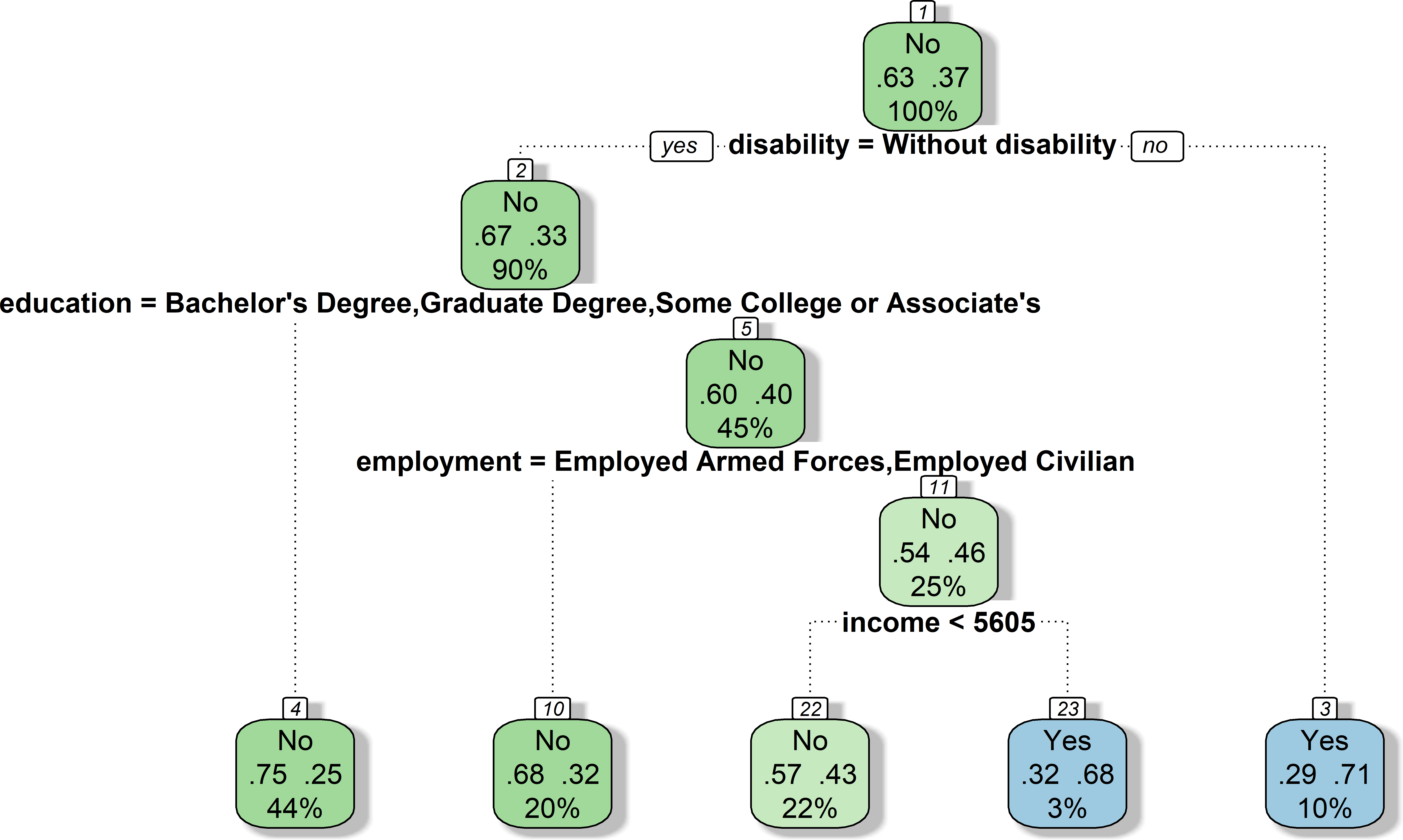
- Let’s quickly review the relevant concepts of a decision tree in Figure 1
- Nodes (with index), majority class, proportion of classes, \(\%\) of original \(n\)
4.1 Model-specific Feature Importance: CART (single tree!)
\[ \mathcal{I}_{\ell}^{2}(T)=\sum \limits_{t=1}^{J-1}\hat{\imath}_{t}^{2}I(\upsilon(t)=\ell) \]Explanations3
calculates total importance of variable \(\ell\) in decision tree by summing up squared reductions in impurity (\(\hat{\imath}_{t}^{2}\)) at each node \(t\) where \(\ell\) is used as splitting variable (the more a variable is used in splitting data, the more important it is for the model)
Classification: Overall reduction of impurity caused by predictor \(X_\ell\)
Regression: Overall reduction in RSS caused by predictor \(X_\ell\)
Importance with Random Forests: Average improvement caused by predictor \(X_\ell\) over all trees4
\[ \mathcal{I}_{\ell}^{2}=\dfrac{1}{M} \sum \limits_{m=1}^{M} \mathcal{I}_{\ell}^{2}(T_{m}) \]
5 Model-Agnostic Importance
- Treat model as a “black box” and can be applied to any trained model
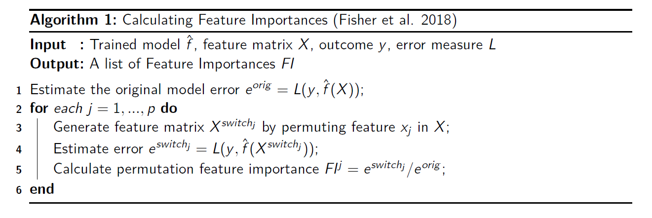
- Permutation Feature Importance (PFI) (Breiman 2001; Fisher, Rudin, and Dominici 2018)
- Train your model and calculate baseline performance score (e.g., accuracy, AUC)
- Take one feature column and randomly shuffle its values, breaking relationship between that feature and the target
- Pass shuffled dataset through (already trained) model again and get new performance score
- “Importance” of feature is the drop in performance from the baseline5
- SHAP (SHapley Additive exPlanations): Cutting-edge method for both global & local explanations (see you later!)
6 Permutation Feature Importance
7 PFI plot
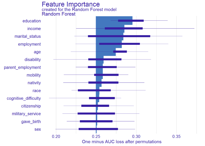
- Interpretation of “PFI plot” in Figure 2
- Point estimate (end of light blue bars) describes the median loss (1 - AUC = area outside the curve) when permutating this feature (repeatedly)
- Dark blue boxplots show results from multiple repeated shuffles for each feature (set in DALEX, e.g.,
B = 10)- Horizontal Lines (Whisker): Show full range of losses for the shuffle results6
8 Feature Importance & Fairness (1)
- Use techniques as diagnostic tool to audit for potential bias
- Direct Discrimination: Check if protected attributes (e.g., gender, race) have high feature importance
- e.g., if model predicting hiring success ranks ‘gender’ highly, it’s a major red flag
- Proxy Detection (Indirect Discrimination): Seemingly neutral feature can be a strong proxy for a protected one
- Example: In a US context, ‘zip code’ can be highly correlated with ‘race’. If your model doesn’t use ‘race’ but heavily relies on ‘zip code’, it can still produce racially biased outcomes
- Q: Can you think of any further examples of protected attributes and/or proxies?
9 Feature Importance & Fairness (2): Audit workflow
- Train your model.
- Calculate global feature importance (e.g., using PFI).
- Analyze the top features: Are any of them protected attributes or potential proxies?
- If a suspicious feature (e.g., ‘zip code’) is highly important, investigate its relationship with protected groups in your data (e.g., race)
- Retrain model without problematic feature and see how performance and fairness metrics change
10 Strenghts and limitations (PFI)
- Strengths
- Limitations
11 Summary & Key Takeaways
- Feature importance tells you what your model is paying attention to
- Model-specific (e.g., coefficients, Gini) vs. model-agnostic (e.g., Permutation, SHAP) methods
- Feature importance relevant for performance but also for fairness auditing
- Question your features: High-ranking feature is a conversation starter
12 Lab R: Feature importance
This lab uses the folktables dataset to predict public health insurance coverage. We will train a model and then use feature importance techniques to audit it for potential biases related to protected attributes like race or sex.
- Goal: Train a model and use feature importance to check for potential biases.
- R Libraries: tidymodels, DALEX, vip, iml
12.1 Prepare data and train model
First, we’ll set up our modeling workflow. This includes selecting the final variables, splitting the data into training and testing sets, defining a recipe for preprocessing, and training a Random Forest model.
- Q: The model below is not very accurate because we don’t tune to speed things up. Is that a problem for interpretability?
library(conflicted)
library(tidyverse)
library(tidymodels)
library(DALEX)
library(vip)
conflicts_prefer(DALEX::explain)
conflicts_prefer(dplyr::select)
conflicts_prefer(yardstick::accuracy)
conflicts_prefer(yardstick::recall)
conflicts_prefer(yardstick::precision)

#data <- read_csv(url(sprintf("https://docs.google.com/uc?id=%s&export=download",
#                         "1dnCK79T45Qa7RZrDg1qv6-EdGBoxCPjv")))

data <- read_csv("data/data_acspubliccoverage.csv")
data <- data %>% mutate(across(where(is.character), as.factor))

# Split the clean data
set.seed(123)
data_split <- initial_split(data, prop = 0.80, strata = public_coverage)
data_train <- training(data_split)
data_test  <- testing(data_split)

# Define the recipe and model spec
recipe_rf <- recipe(public_coverage ~ ., data = data_train) %>%
  step_impute_median(all_numeric_predictors()) %>% # Impute numeric NAs
  step_impute_mode(all_nominal_predictors())      # Impute categorical NAs
model_rf <- rand_forest(mode = "classification") %>%
  set_engine("ranger", importance = "impurity")

# Create and fit the workflow
workflow_rf <- workflow() %>%
  add_recipe(recipe_rf) %>%
  add_model(model_rf)
fit_rf <- fit(workflow_rf, data = data_train)

# fit_rf_test <- fit(workflow_rf, data = data_test)

# Test data: Metrics
   metrics_combined <- metric_set(accuracy,
                                  recall,
                                  precision,
                                  f_meas)
  data_test %>%
    augment(x = fit_rf, type.predict = "response") %>%
      metrics_combined(truth = public_coverage, estimate = .pred_class) # how could we change the threshold?
# A tibble: 4 × 3
.metric .estimator .estimate
<chr> <chr> <dbl>
1 accuracy binary 0.714
2 recall binary 0.883
3 precision binary 0.726
4 f_meas binary 0.79712.2 Task 1: Model-Specific Importance
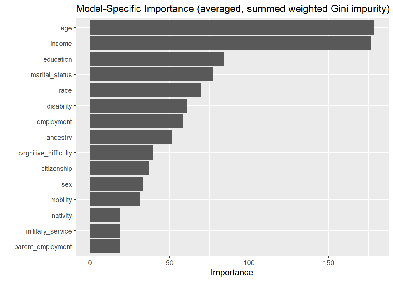
Let’s start by looking at the importance metric that is built into the random forest algorithm itself (Gini impurity).
- Instructions: Use the
vippackage, which is part of thetidymodelsecosystem, to extract and plot the built-in feature importance. - Discussion Question: What does the model think is most important? Are there any surprises?
12.3 Task 2: Model-Agnostic Importance (Permutation)
Model-specific importance can sometimes be biased. A more reliable method is permutation feature importance (PFI), which is model-agnostic and calculated on unseen test data.
- Instructions: Use the
DALEXpackage to compute and plot permutation feature importance on the test set.15explain(): creates a unified representation of a model, which can be further processed by functions for explanationsmodel_parts(): Estimates dataset level variable importance as change in loss function after Variable permutations- Default loss_function is \(1 - \text{AUC(= area under the curve)}\), i.e., how much the model’s performance worsens when feature is shuffled
- Discussion Question: How do these results compare to the built-in importance? Do the top features change?
# First, create a DALEX explainer for our fitted workflow
p_fun <- function(object, newdata) {
  predict(object, new_data = newdata, type = "prob")$.pred_Yes
}

explainer <- explain(
  model = fit_rf,
  data = select(data_test, -public_coverage),
  y = as.numeric(data_test$public_coverage == "Yes"),
  predict_function = p_fun,
  label = "Random Forest",
  type = "classification",
  verbose = FALSE
)

# Now, calculate and plot permutation feature importance
# DALEX's model_parts() calculates PFI by default.
pfi <- model_parts(explainer,
                   N = 100,
                   B = 10) # number of observations sampled for calculation

plot(pfi, max_vars = 15)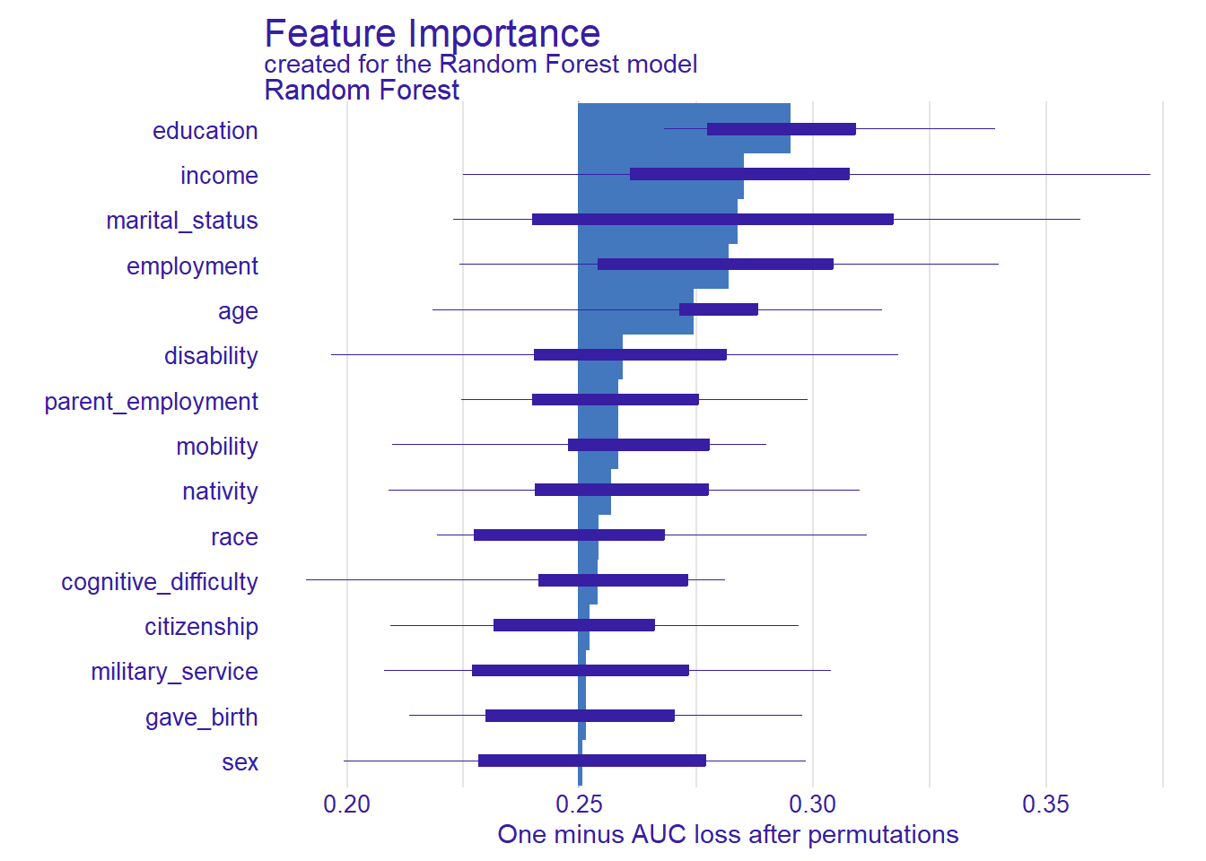
12.4 Task 3: Fairness Analysis
Now we use the more reliable permutation importance plot from Task 2 to look for potential fairness issues.
- Critical Thinking & Fairness Discussion:
- Look at your final importance plot (
DALEXPFI). Where dosexandracerank? Are they in the top 10? - High importance for features like
incomeandagemakes sense for predicting health care insurance coverage. But look at other high-ranking features. Could any of them be proxies for protected characteristics? For example, couldmarital_statusoreducationbe correlated with gender or race in a way that disadvantages a certain group?
- Look at your final importance plot (
12.5 Task 4: Bias Mitigation
A key step in mitigating bias is to see what happens when you remove a protected attribute.
- Instructions: Create a new model trained on data without the
racevariable and see how the feature importances change. - Discussion: Did the importance of other variables change? Sometimes, when a protected attribute is removed, the model will “shift” the importance to other variables that are correlated with it (proxies). This is a crucial effect to watch for.
# 1. Create a new recipe that removes the race variable
recipe_rf_no_race <- recipe(public_coverage ~ ., data = data_train %>% select(-race)) %>%
  step_impute_median(all_numeric_predictors()) %>% # Impute numeric NAs
  step_impute_mode(all_nominal_predictors())      # Impute categorical NAs

# 2. Create and fit a new workflow & prepare data
workflow_rf_no_race <- workflow_rf %>%
  update_recipe(recipe_rf_no_race)

  fit_rf_no_race <- fit(workflow_rf_no_race, data = data_train)

 # Bake data_test with new recipe
  recipe_prepped <- prep(recipe_rf_no_race, training = data_train) # estimate required parameters from training set to use on test data
  test_data_baked <- bake(recipe_prepped, new_data = data_test)

# 3. Create a new explainer for the new model
explainer_no_race <- explain(
  model = fit_rf_no_race,
  data = select(test_data_baked, -public_coverage),
  y = as.numeric(data_test$public_coverage == "Yes"),
  predict_function = p_fun,
  label = "Random Forest (No race)",
  type = "classification",
  verbose = FALSE
)

# 4. Calculate and plot the new permutation importance
pfi_rf_no_race <- model_parts(explainer_no_race, N = 100)
plot(pfi_rf_no_race, max_vars = 15)
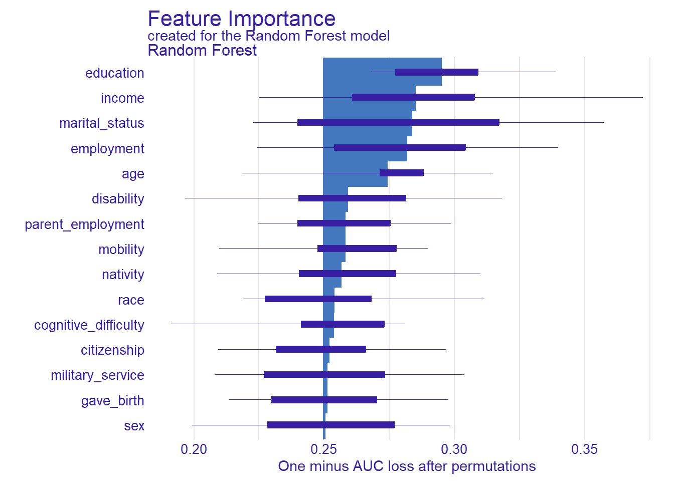
plot(pfi, max_vars = 15)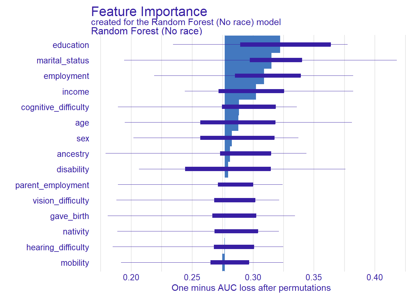
12.6 Exercise R
- Above we investigated feature importance (specific and agnostic using the PFI). We identified, e.g.,
marital_statusas a problematic variable. Please restimate the model now excludingmarital_status. - Create two graphs for model-specific importance and the PFI. Do you observe any changes?
Answer/Solution(s)
- Exercise 1
library(tidyverse)
library(tidymodels)
library(DALEX)
library(vip)
library(yardstick)


#data <- read_csv(url(sprintf("https://docs.google.com/uc?id=%s&export=download",
#                         "1dnCK79T45Qa7RZrDg1qv6-EdGBoxCPjv")))

data <- read_csv("data/data_acspubliccoverage.csv")
data <- data %>% mutate(across(where(is.character), as.factor))

# Split the clean data
set.seed(123)
data_split <- initial_split(data, prop = 0.80, strata = public_coverage)
data_train <- training(data_split)
data_test  <- testing(data_split)

# Define the recipe and model spec
recipe_rf <- recipe(public_coverage ~ ., data = data_train %>% select(-marital_status)) %>%
  step_impute_median(all_numeric_predictors()) %>% # Impute numeric NAs
  step_impute_mode(all_nominal_predictors())      # Impute categorical NAs

model_rf <- rand_forest(mode = "classification") %>%
  set_engine("ranger", importance = "impurity")

# Create and fit the workflow
workflow_rf <- workflow() %>%
  add_recipe(recipe_rf) %>%
  add_model(model_rf)
fit_rf <- fit(workflow_rf, data = data_train)

# Test data: Metrics
   metrics_combined <- metric_set(yardstick::accuracy,
                                  yardstick::recall,
                                  yardstick::precision,
                                  yardstick::f_meas)
  data_test %>%
    augment(x = fit_rf, type.predict = "response") %>%
      metrics_combined(truth = public_coverage, estimate = .pred_class)
# A tibble: 4 × 3
.metric .estimator .estimate
<chr> <chr> <dbl>
1 accuracy binary 0.714
2 recall binary 0.893
3 precision binary 0.722
4 f_meas binary 0.799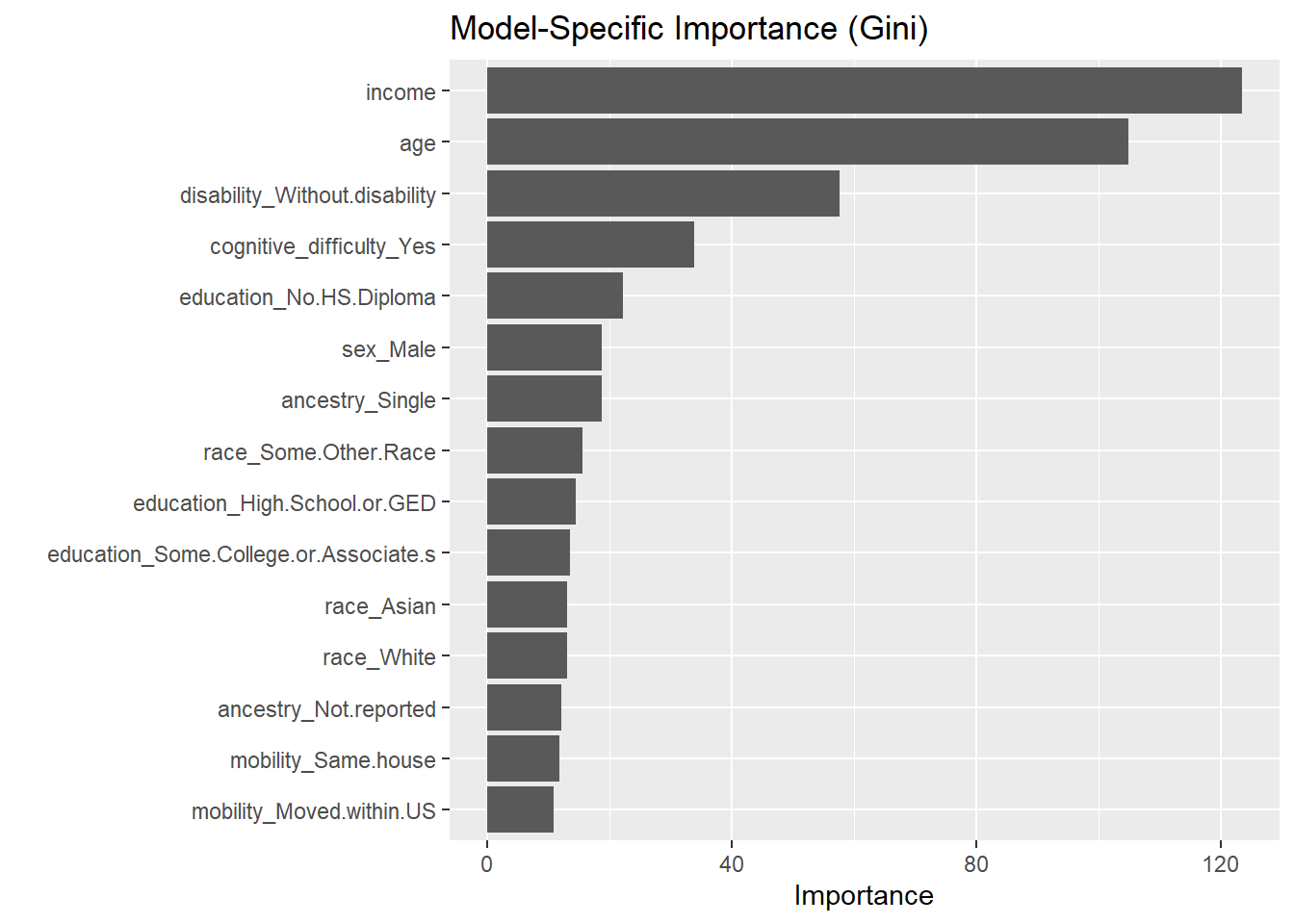
# First, create a DALEX explainer for our fitted workflow
p_fun <- function(object, newdata) {
  predict(object, new_data = newdata, type = "prob")$.pred_Yes
}

explainer <- explain(
  model = fit_rf,
  data = select(data_test, -public_coverage),
  y = as.numeric(data_test$public_coverage == "Yes"),
  predict_function = p_fun,
  label = "Random Forest",
  type = "classification",
  verbose = FALSE
)

# Now, calculate and plot permutation feature importance
# DALEX's model_parts() calculates PFI by default.
pfi <- model_parts(explainer, N = 100) # Use a sample for speed

plot(pfi, max_vars = 15)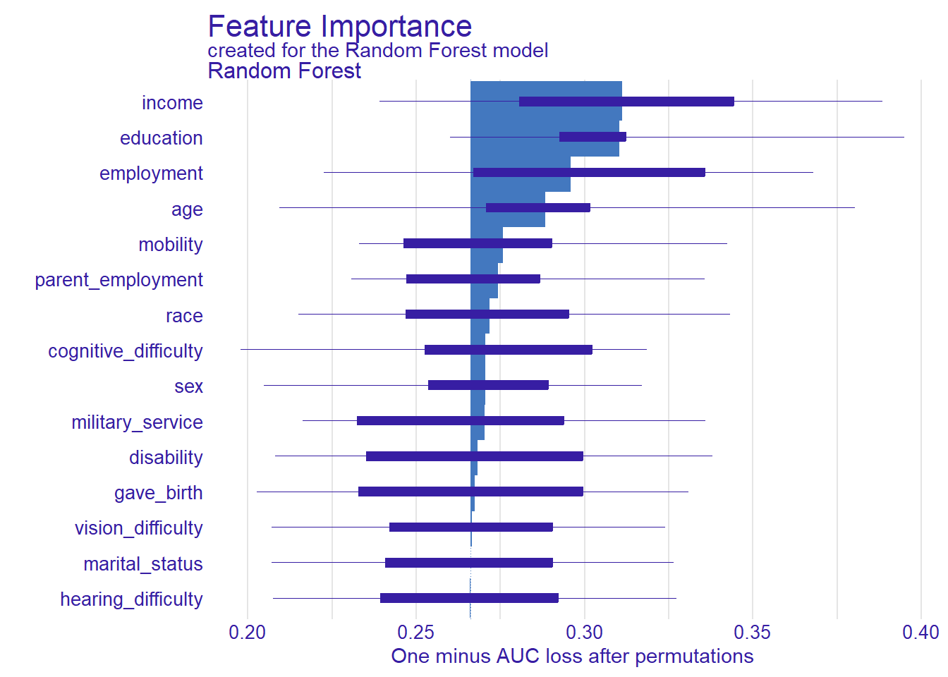
12.7 Appendix: iml package
- Use the
imlpackage to compute and plot permutation feature importance on the test set.Predictor: creates a unified representation of a model, which can be further processed by functions for explanationsFeatureImp: Estimates dataset level variable importance as change in loss function after Variable permutations- Default loss function is ce = classification error = 1 - accuracy
- x-axis measures ratio of the model’s error after feature is shuffled to the model’s original error
- e..g, value of 1.08 means that shuffling the feature caused the model’s classification error to increase by 8%
- Default loss function is ce = classification error = 1 - accuracy
library(conflicted)
library(tidyverse)
library(tidymodels)
library(DALEX)
library(vip)
conflicts_prefer(DALEX::explain)
conflicts_prefer(dplyr::select)
conflicts_prefer(yardstick::accuracy)
conflicts_prefer(yardstick::recall)
conflicts_prefer(yardstick::precision)

#data <- read_csv(url(sprintf("https://docs.google.com/uc?id=%s&export=download",
#                         "1dnCK79T45Qa7RZrDg1qv6-EdGBoxCPjv")))

data <- read_csv("data/data_acspubliccoverage.csv")
data <- data %>% mutate(across(where(is.character), as.factor))

# Split the clean data
set.seed(123)
data_split <- initial_split(data, prop = 0.80, strata = public_coverage)
data_train <- training(data_split)
data_test  <- testing(data_split)

# Define the recipe and model spec
recipe_rf <- recipe(public_coverage ~ ., data = data_train) %>%
  step_impute_median(all_numeric_predictors()) %>% # Impute numeric NAs
  step_impute_mode(all_nominal_predictors())      # Impute categorical NAs
model_rf <- rand_forest(mode = "classification") %>%
  set_engine("ranger", importance = "impurity")

# Create and fit the workflow
workflow_rf <- workflow() %>%
  add_recipe(recipe_rf) %>%
  add_model(model_rf)
fit_rf <- fit(workflow_rf, data = data_train)

# fit_rf_test <- fit(workflow_rf, data = data_test)

# Test data: Metrics
   metrics_combined <- metric_set(accuracy,
                                  recall,
                                  precision,
                                  f_meas)
  data_test %>%
    augment(x = fit_rf, type.predict = "response") %>%
metrics_combined(truth = public_coverage, estimate = .pred_class) # how could we change the threshold?library(iml)
# 1. Create an iml Predictor object for the fitted workflow
# This object wraps the model and data for the iml package.
class_fun <- function(object, newdata) {
predict(object, new_data = newdata, type = "class")$.pred_class
}
predictor <- Predictor$new(
model = fit_rf,
data = dplyr::select(data_test, -public_coverage), # Predictor variables from test set
y = data_test$public_coverage, # Outcome variable from test set
predict.function = class_fun,
type = "classification" # Specify the task type
)
# 2. Calculate and plot permutation feature importance
# The FeatureImp$new() function calculates PFI. The default loss for
# classification is classification error (1 - accuracy).
pfi_iml <- FeatureImp$new(predictor, loss = "ce")
# Plot the results, showing the top 15 features
plot(pfi_iml, n.features = 15)13 Lab Python
Overview: https://docs.google.com/document/d/1mUDDwZMZR-9aRZhvSzDEC85sXmwOMB4Y8okMXbehytY/
References
Breiman, L. 2001. “Random Forests.” Machine Learning 45: 5–32.
Fisher, Aaron, C Rudin, and F Dominici. 2018. “All Models Are Wrong, but Many Are Useful: Learning a Variable’s Importance by Studying an Entire Class of Prediction Models Simultaneously.” Journal of Machine Learning Research: JMLR 20.
Molnar, Christoph. 2022. “Interpretable Machine Learning.” https://christophm.github.io/interpretable-ml-book/.
Molnar, Christoph, Gunnar König, Julia Herbinger, Timo Freiesleben, Susanne Dandl, Christian A Scholbeck, Giuseppe Casalicchio, Moritz Grosse-Wentrup, and Bernd Bischl. 2022. “General Pitfalls of Model-Agnostic Interpretation Methods for Machine Learning Models.” In xxAI - Beyond Explainable AI, 39–68. Springer International Publishing.
Footnotes
Global interpretation methods: describe the expected behavior of the entire model with respect to the whole data distribution. Local explanation methods: explain individual predictions or classifications. Feature importance methods: quantify the contribution of a feature to the model performance (e.g. via a loss function) or to the variance of the prediction function. Effect methods: indicate the direction and magnitude of a change in predicted outcome due to changes in feature values (Molnar et al. 2022, 40–41).↩︎
Impurity reduction is the benefit gained from a split, measured as the decrease in data “mixed-ness” from before the split to after. Gini impurity, calculates the probability of misclassifying a randomly chosen element from a group if it were labeled according to the class distribution within that group. \(\text{Gini Impurity}\) \(=\) \(p(No) * (1- p(No))\) \(+ p(Yes) * (1-p(Yes))\) \(= 0.67 * (1 - 0.67)\) \(+ 0.33 * (1 - 0.33)\) \(= 0.44\).↩︎
…where \(\mathcal{I}_{\ell}^{2}(T)\) is the importance score of the variable \(\ell\) in the decision tree \(T\)
\(\sum \limits_{t=1}^{J-1}\) sums up the importance of a predictor/variable \(\ell\) across all the nodes \(t\) where it was used for splitting (\(J\) being the total number of nodes)
\(\hat{\imath}_{t}^{2}\) is the (squared) impurity reduction associated with a split at node \(t\)
\(I(\upsilon(t)=\ell)\) is an indicator function (\(= 1\) if the variable \(\ell\) is used in the split at node \(t\), \(0\) otherwise).↩︎Notation: \(\mathcal{I}_\ell\) is the importance of feature \(X_\ell\) in the Random Forest model; \(\mathcal{I}_\ell^2(T_m)\) is the feature importance of feature \(X_\ell\) in a single tree \(T_m\), which measures the improvement in model performance (e.g., reduction in impurity or error) due to feature \(X_\ell\) in tree \(T_m\); \(M\) is the total number of trees in the Random Forest.↩︎
Big drop → model was heavily relying on that feature↩︎
Short whiskers = higher stability, Long whiskers = lower stability.↩︎
PFI provides a global insight into the model by defining importance as the increase in model error observed when a feature’s information is destroyed (by shuffling its values).↩︎
By permuting a feature, the method automatically destroys its interaction effects with other features. This means PFI accounts for both the main feature effect and all interaction effects on model performance.↩︎
PFI does not require the model to be retrained. Other methods that involve deleting a feature and retraining can be very time-consuming, so “only” permuting a feature saves a lot of time.↩︎
Because PFI is linked to the model’s loss, it is great for data insights. If a feature is irrelevant for predicting the outcome (but is still used by the model for overfitting), PFI will correctly show an importance near zero.↩︎
This is the primary limitation. Permuting one of two correlated features creates unrealistic data instances (e.g., a 2-meter tall person weighing 30kg). The model’s error on these impossible instances biases the importance score. This can also “split” the importance, making two important, correlated features both appear mediocre.↩︎
PFI is just a ranking. It tells you how much a feature impacts the model’s error, but not how it influences the prediction (e.g., whether increasing the feature increases or decreases the outcome).↩︎
You cannot compute PFI if you only have the model and unlabeled data. You must have access to the true outcomes (labels) to calculate the change in model error.↩︎
The shuffling process adds randomness to the measurement. If the permutation is not repeated and averaged, the results can vary greatly between runs, which can be misleading. Most software implementations repeat and average the permutations.↩︎